Lab 6 RNA-seq analysis

6.1 Objectives

After this section you should be able to:

1. Understand RNA sequencing counts.
2. Perform distance matrix and PCA.
3. Do differential gene expression using DeSeq2.

6.2 Introduction

We will re-analyze some data from Abruzzi et al, 2017. These are data that explore gene expression in different neuronal cell types in a circadian layout.

This time we will just take the process data from the paper, and no directly the Raw data like in the previous chapter (Chip-seq). The data was downloaded from GEO. The only pre-processing to the data was done to change column names.

As you can see in the methods section of the paper they have different cell-types and timepoints. Let’s try to understand what type of system and data we have in hands.

Circadian behavior

Most living organisms change their behavior and metabolism over the day. Some animals like us have more activity over the day while others like mice have more activity over night. Flies in particular have a peak of activity the first hours of the morning and the last hours of the afternoon with a “siesta” (nap in Spanish) at the middle of the day.

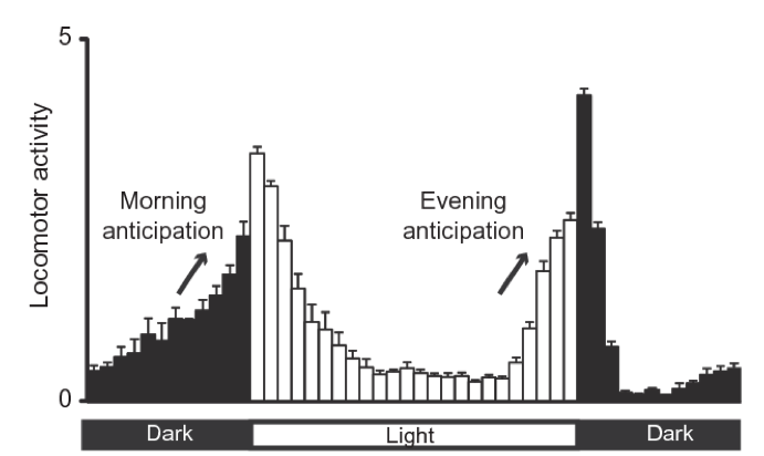
Figure 4.1: Fly activity over the day. Adapted from Nicholas R. J Glossop et al 2011. To meassure fly activity each individual fly is monitored either by counting when they cross a red-light bim (regular activity monitors) of by software tracking (flyboxes).

These changes in behavior are govern by changes in gene expression in particular cell-types in the brain called the pace-makers. If we look at gene expression in these cells over the day we will notice that some genes oscillate. Like Clk and tim, the proteins we analyzed in the previous Lab.

In the circadian field time is reported as “hours after the light is ON”. This is zeitgeber time (ZT) and it is useful to have a unified measurement of time. Most animals in labs are kept in 12 hours of light followed by 12 hours of dark. Therefore, ZT0 is the “sunrise” or lights on and ZT12 is lights off in a light/dark (LD)12:12 cycle time.

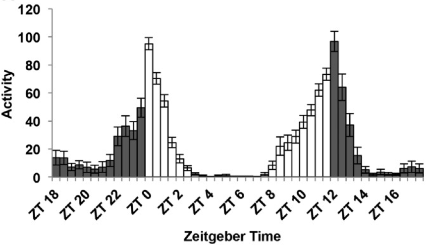
Figure 4.2: Fly activity over the day with ZT scale. Figure adapted from Dubowy et al 2017

As stated before, circadian behaviors is generated by a small subset of neurons.

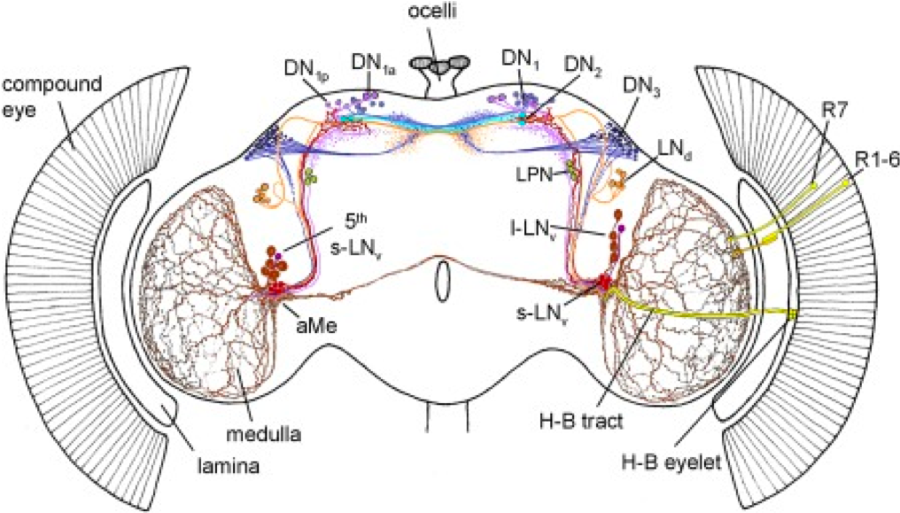
Figure 4.3: Schematic representation of the circadian neural network. Four small ventrolateral neurons (s‐LNvs, red), the 5th s‐LNv (dark violet), four large ventrolateral neurons (l‐LNvs, brown), six dorsolateral neurons (LNds, orange), three lateral posterior neurons (LPN, green), and ca. 60 neurons per hemisphere in three dorsal groups (DN1–3, lilac, cyan, blue, respectively). Adapted from Schubert et al 2018

In the data analyzed in this lab, the authors collected RNA samples over 6 times of the day (ZT3, 7, 11, 15, 19, 23) from 4 cell-types: LNv, LNd, DN1 and Dopaminergic neurons (TH cells). This last group of cells are not part of the circadian core clock but in this study they see oscillating genes!

Packages:

We will use the following packages. Do not forget to executing them every time you open a new R session. Before running them for the first time, you will have to install them (go back to Lab1 if you have any doubt).

library(DESeq2) #for differential expression analysis
library(ggplot2) #for 2D graph
library(ggrepel) #to get the names in ggplot graph 
library(gridExtra) #to arrange the plots
library(factoextra) #extra plots
library(plotly) #for 3D graphics
library(plyr) #table manipulation
library(dplyr)#table manipulation
library(tidyr)#table manipulation
library("RColorBrewer") #extra color palettes
library("pheatmap") #nice heatmaps
library(org.Dm.eg.db) #get annotation
library(MetaCycle) # to identify cycling genes, the successor of JTK according to JTK authors
library(pcaExplorer) #more PCA analysis

6.3 Differential gene expression

Gene expression data is made of integer numbers by genes. Each number represents exactly how many reads aligned to the DNA sequence that is assigned to each gene.

Gene counts table

Gene	Condition 1 replicate 1	Condition 1 replicate 2	Condition 2 replicate 1	Condition 2 replicate 2
A	20	400	60	40
B	2	50	2000	2500
C	0	5	0	0
D	5	2050	150	144

Ultimately, what we want to do is to compare gene expression between conditions. To do so we have to make some considerations. One is the fact that we want to make conclusions about the whole transcriptome of the organism we are working with. This means around 12000 comparisons (assuming 12000 genes). This implies a huge multiple-comparison correction. Another important consideration is the difference in sequencing depth, to overcame this issue the reads are normalized using an estimate that includes the total amount of reads in that sample. Finally, genes that are too lowly expressed or have a huge dispersion have to be removed from the analysis as they are too noisy to get a trustable conclusion from them.

To perform differential gene expression, we have to build a model that explains the differences in gene expression using the condition we are testing, fit the data to that model and see if it can explain the differences. This is done using generalized linear models (GLM) modeled using a negative binomial distribution (NB). Why is this? Because the data are counts, ie. integers (there are not 12.5 reads, you either have 12 or 13), to model discrete counts, we use either poison or NB distribution. NB is used because it allows for expression and variance to be unlinked.

Luckily for us, there are many packages dedicated to solve this problem. We will use DeSeq2

The steps performed by the DESeq function are documented in the manual page of DESeq2; briefly, they are:

1 estimation of size factors by estimateSizeFactors (this is for normalization) 2 estimation of dispersion by estimateDispersions (calculate the gene expression dispersion) 3 negative binomial GLM fitting and Wald statistics by nbinomWaldTest (this is the actual differential gene expression step)

The only requirement for Deseq2 is to have the tables of data in a proper format and a meta-data object that indicates what is each sample.

Imagine we have a wildtype and a mutant, DeSeq2 requires Table: 1: Data matrix with Gene name as ROWNAMES

2: MetaData (colData) in which ROWNAMES are the COLNAMES of the Data matrix and the conditions are column names

Row Names	WildType.1	WildType.2	Mutant.1	Mutant.2
geneA	20	400	60	40
geneB	2	50	2000	2500
geneC	0	5	0	0
geneD	5	2050	150	144

Row Names	Genotype	replicate
WildType.1	WT	1
WildType.2	WT	2
Mutant.1	actinKD	1
Mutant.2	actinKD	2

The we can use the Genotype as a condition to compare gene expression for example.

At this time, we will start by comparing gene expression at two timepoints in one cell-type. This is good to have a first impression of the data but it is not the way to go if your idea is to analyze circadian cycling behavior.

6.3.1 Loading the tables

This time we have 4 gene expression tables: one for each cell type we are analyzing. Therefore, some of the processing will be done using for loops. This might be confusing at the beginning but is a really useful tool.

#We can list the files that are present in our working directory, or any path we specify. Remember the path will change depending where you have your data.
list.files(path = "../RNAseq/")
list.files(path = "../RNAseq/",pattern = "expression") #what do you think patter is doing? remember to go to the help page if you need to.
list.files(path = "../RNAseq/",pattern = "expression",full.names = T) #what happened now?

paper_tables<-list.files(path = "../RNAseq/",pattern = "xpression",full.names = T) #what we are doing here?, check your environment, do you see something new?

#If we try with one
TH_gene_expression<-read.table("../RNAseq/TH_gene_expression.txt",header = T)

##  [1] "all_tables.rdata"        "circadianact.png"       
##  [3] "circadianbrain.png"      "circadiancells.png"     
##  [5] "cycDN1_reults.txt"       "cycDN1.csv"             
##  [7] "cycwithzt.png"           "DN1_gene_expression.txt"
##  [9] "F1.large.jpg"            "howcircadian.png"       
## [11] "LNd_gene_expression.txt" "LNv_gene_expression.txt"
## [13] "RNASeq_DeSeq2.html"      "RNASeq_DeSeq2.rmd"      
## [15] "RNAseqDataPrep.html"     "TableMod.rmd"           
## [17] "TH_gene_expression.txt" 
## [1] "DN1_gene_expression.txt" "LNd_gene_expression.txt"
## [3] "LNv_gene_expression.txt" "TH_gene_expression.txt" 
## [1] "../RNAseq//DN1_gene_expression.txt" "../RNAseq//LNd_gene_expression.txt"
## [3] "../RNAseq//LNv_gene_expression.txt" "../RNAseq//TH_gene_expression.txt"

How can we make it work for all the tables? We want to change the name, we basically want to remove the “.txt” ending. That can be done using gsub. We want to remove “.txt”, so we replace it for an empty string.

gsub(x = "../RNAseq/TH_gene_expression.txt",pattern =".txt",  replacement = "")

## [1] "../RNAseq/TH_gene_expression"

#We also need to remove the path file
gsub(x = "../RNAseq/TH_gene_expression.txt",pattern ="../RNAseq/",  replacement = "")

## [1] "TH_gene_expression.txt"

Now we can try to do it for all of them, just trying to see if changing the names is working but NOT applying it to anything until we know it works.

for (e in (paper_tables)){
  print("original name:          ")
  print(e) # this is printing e
  n<-gsub(pattern =".txt",  replacement = "",x = e)
  n<-gsub(pattern ="../RNAseq//",  replacement = "",x = n)
  print("final name:        ")
  print(n)
}

## [1] "original name:          "
## [1] "../RNAseq//DN1_gene_expression.txt"
## [1] "final name:        "
## [1] "DN1_gene_expression"
## [1] "original name:          "
## [1] "../RNAseq//LNd_gene_expression.txt"
## [1] "final name:        "
## [1] "LNd_gene_expression"
## [1] "original name:          "
## [1] "../RNAseq//LNv_gene_expression.txt"
## [1] "final name:        "
## [1] "LNv_gene_expression"
## [1] "original name:          "
## [1] "../RNAseq//TH_gene_expression.txt"
## [1] "final name:        "
## [1] "TH_gene_expression"

What is this for loop doing? Do you think it is working? Why?

Now we will read the tables and put them in the names we created. To do this we will use the function assign, that actually assign anything to a given name. The name is stored in “n”. What we want to assign is the “read.delim” of the file name stored in e.

for (e in (paper_tables)){
  n<-gsub(pattern =".txt",  replacement = "",x = e)
  n<-gsub(pattern ="../RNAseq//",  replacement = "",x = n)
  print(paste0("I am reading: ",n))
  assign(n,read.delim(e))
}

## [1] "I am reading: DN1_gene_expression"
## [1] "I am reading: LNd_gene_expression"
## [1] "I am reading: LNv_gene_expression"
## [1] "I am reading: TH_gene_expression"

6.3.2 Create the DeSeq2 count matrix

DeSeq2 expects to have a data.frame with the gene-names as row.names and then just the counts.

I will first show it for one of the tables and then do a for loop to do it for all of them.

#We do not want to overwrite the raw tables. So, we will create new objects with the same data and we will modify these new objects and preserve the original data. Is like doing "save as" in word.

ds2_DN1_gene_expression_try<-DN1_gene_expression #what is this doing?

#We do now the loop for all of them to create the `ds2_` objects
ls(pattern = "gene_expression") #this list the objects in the environment that has the selected pattern in its name

## [1] "DN1_gene_expression"         "ds2_DN1_gene_expression_try"
## [3] "LNd_gene_expression"         "LNv_gene_expression"        
## [5] "TH_gene_expression"

#The new name we want is just adding "ds2_" to the beginning of the object name. We can do this with the paste0 function.
paste0("ds2_","DN1_gene_expression")

for (e in ls(pattern = "gene_expression")){ 
  x = paste0("ds2", sep="_",e) #this is the new name
  print("new name is:")
  print(x) 
  assign(x, get(e)) #get is a function that extracts the data from an object name
}

## [1] "ds2_DN1_gene_expression"
## [1] "new name is:"
## [1] "ds2_DN1_gene_expression"
## [1] "new name is:"
## [1] "ds2_ds2_DN1_gene_expression_try"
## [1] "new name is:"
## [1] "ds2_LNd_gene_expression"
## [1] "new name is:"
## [1] "ds2_LNv_gene_expression"
## [1] "new name is:"
## [1] "ds2_TH_gene_expression"

Now we have to do some manipulation in the tables for them to work with Deseq2.

ds2_DN1_gene_expression_try <- ds2_DN1_gene_expression
row.names(ds2_DN1_gene_expression_try) = ds2_DN1_gene_expression$Symbol # we put the symbols as row.names
ds2_DN1_gene_expression_try<-ds2_DN1_gene_expression_try[,-1] # we take the symbols column out
head(ds2_DN1_gene_expression_try) # we can see that now the table is what we need
rm(ds2_DN1_gene_expression_try) #remove it because you do not need it anymore and because it can create problems

##             DN1_ZT3_1 DN1_ZT7_1 DN1_ZT11_1 DN1_ZT15_1 DN1_ZT19_1 DN1_ZT23_1
## FBtr0070202         0         0          0          0          0          0
## FBtr0070207         0         0          0          0         14          0
## FBtr0070238         0         0          0          0         21          0
## FBtr0070251         0         0          0          0          0          0
## FBtr0070484         0         0          0          0          0          0
## FBtr0070489         0         0          0          0          0          0
##             DN1_ZT3_2 DN1_ZT7_2 DN1_ZT11_2 DN1_ZT15_2 DN1_ZT19_2 DN1_ZT23_2
## FBtr0070202         0         0          0          0          0          0
## FBtr0070207         0         0          0          0         16          7
## FBtr0070238         0         0          0          0         15          9
## FBtr0070251         0         0          1          0          2          0
## FBtr0070484         0         0          0          0          0          1
## FBtr0070489         0         0          0          0          0          0

We can add this step to the for loop, or even better we can create a function and practice something new in R.

#We create a small function to remember
sum2<-function(x){
 y=x+2 
 return(y)
}

sum2(4) 

## [1] 6

what is this doing? why?

#Now we create a function that takes the data frame and does all the transformation we did before
create_ds2= function(df_name){
  df = as.data.frame(get(df_name))
  row.names(df) = as.character(df[,1])
  df=df[,-1]
  return(df) # this actually tells the function to return the transformed data.frame
}

#Let's try the function in one of the ds2 objects
#head(create_ds2(ds2_LNd_gene_expression))[,c(1:3)]
for (e in ls(pattern = "ds2_")){
  print(e)
  assign(e,create_ds2(e)) #this should actually run the function and apply it to the data frame
}

## [1] "ds2_DN1_gene_expression"
## [1] "ds2_ds2_DN1_gene_expression_try"
## [1] "ds2_LNd_gene_expression"
## [1] "ds2_LNv_gene_expression"
## [1] "ds2_TH_gene_expression"

6.3.3 Meta-data (colData) preparation

We now need to have a data.frame with the mapping between the columns and the ZT, the program call this colData. Is what is usually called “meta data”. Is a file that explains what each object/column is.

We will do it by hand just changing the names. No more loops for now. After you execute each step I recommend you to inspect the object to see what is happening.

DN1

#takes the names in the data frame and put them in the new objects. We want to get the information for each 
colData.DN1 = as.data.frame(names(ds2_DN1_gene_expression)) 
#now we put them as row.names
rownames(colData.DN1) = colData.DN1[,1]
#now we take the columns out 
colData.DN1 =colData.DN1[,-1]
#this is taking the last part of the rownames and put them in a column named `ZT`
colData.DN1$ZT = sapply(strsplit(rownames(colData.DN1),"_"),"[[",2)
colData.DN1$rep = sapply(strsplit(rownames(colData.DN1),"_"),"[[",3)

head(colData.DN1)

##              ZT rep
## DN1_ZT3_1   ZT3   1
## DN1_ZT7_1   ZT7   1
## DN1_ZT11_1 ZT11   1
## DN1_ZT15_1 ZT15   1
## DN1_ZT19_1 ZT19   1
## DN1_ZT23_1 ZT23   1

LNv

colData.LNv = as.data.frame(names(ds2_LNv_gene_expression)) 
#now we put them as row.names
rownames(colData.LNv) = colData.LNv[,1]
#now we take the columns out 
colData.LNv =colData.LNv[,-1]
#this is taking the last part of the rownames and put them in a column named `ZT`
colData.LNv$ZT = sapply(strsplit(rownames(colData.LNv),"_"),"[[",2)
colData.LNv$rep = sapply(strsplit(rownames(colData.LNv),"_"),"[[",3)

LNd

colData.LNd = as.data.frame(names(ds2_LNd_gene_expression)) 
#now we put them as row.names
rownames(colData.LNd) = colData.LNd[,1]
#now we take the columns out 
colData.LNd =colData.LNd[,-1]
#this is taking the last part of the rownames and put them in a column named `ZT`
colData.LNd$ZT = sapply(strsplit(rownames(colData.LNd),"_"),"[[",2)
colData.LNd$rep = sapply(strsplit(rownames(colData.LNd),"_"),"[[",3)

TH

colData.TH = as.data.frame(names(ds2_TH_gene_expression)) 
#now we put them as row.names
rownames(colData.TH) = colData.TH[,1]
#now we take the columns out and 
colData.TH =colData.TH[,-1]
colData.TH$ZT = sapply(strsplit(rownames(colData.TH),"_"),"[[",2)
colData.TH$rep = sapply(strsplit(rownames(colData.TH),"_"),"[[",3)

6.3.4 Quality filtering: Distance matrix and principal component analysis (PCA)

If we want to evaluate the difference between two conditions we have to make sure that the difference between replicates of the same conditions are smaller. In other words, we expect the replicates of the same condition to be similar to each other. Checking this is a regular procedure in differential gene expression analysis as it helps us to identify samples that might be outliers.

To evaluate this, we will use two different approaches. Firstly, we will calculate a distance matrix, this is basically calculating the difference between each sample. To visualize this, we will use a heatmap. Secondly, we will do a principal component analysis (PCA) to get an idea on how similar are the samples between each other. To make it simple (but not completely correct) PCA is a way to reduce the dimensions (in this case many many genes) to a set of vectors (principal components, PC) that summarize the combination of the gene information. Then, if two samples have similar values in this PCs then they are similar to each other.

We first have to initiate the DeSeq2 object. This imply telling the package which is the matrix of read counts, the colData (meta data) and the design. The design is what the program uses to do the differential expression. Is simple in this case: only the ZT.

Initialize the data

#This is actually the main function of the package and prepares everything to run the differential expression analysis.
dds.DN1 <- DESeqDataSetFromMatrix(countData = as.matrix(ds2_DN1_gene_expression), colData = colData.DN1,design = ~ ZT)

#class of dds.DN1
class(dds.DN1)

## [1] "DESeqDataSet"
## attr(,"package")
## [1] "DESeq2"

Distance Matrix

As stated before, a distance matrix is a way to quantify differences. In this case each column of the data matrix will be compared with all the others. You can read more here or here. dist() is the function that calculates the Euclidean distance, you can select which type of distance you want to calculate, read the help page for more information.

# Calculate the distance matrix
sampleDists <- dist(t(assay(dds.DN1))) 

# Lets look at this step by step:
# assay(dds.DN1) # extract the reads
# t(assay(dds.DN1)) #transpose the matrix, this has to do with the fact that we want to calculate the distance between samples, if we do not transpose we will literally calculate the difference between genes across samples

#Then we take this in a matrix and create the heatmap
sampleDistMatrix <- as.matrix(sampleDists) #convert to matrix

rownames(sampleDistMatrix) <- paste(dds.DN1$ZT,dds.DN1$rep,sep="_rep_") # put the rownames
colnames(sampleDistMatrix) <- NULL
colors <- colorRampPalette( rev(brewer.pal(9, "Blues")) )(255)#select color 

#Heatmap function
pheatmap(sampleDistMatrix,
         clustering_distance_rows=sampleDists,
         clustering_distance_cols=sampleDists,
                  annotation_row = rownames(sampleDists),
         annotation_col = rownames(sampleDists),
         cutree_rows = 2,
         cutree_cols = 2,
         col=colors)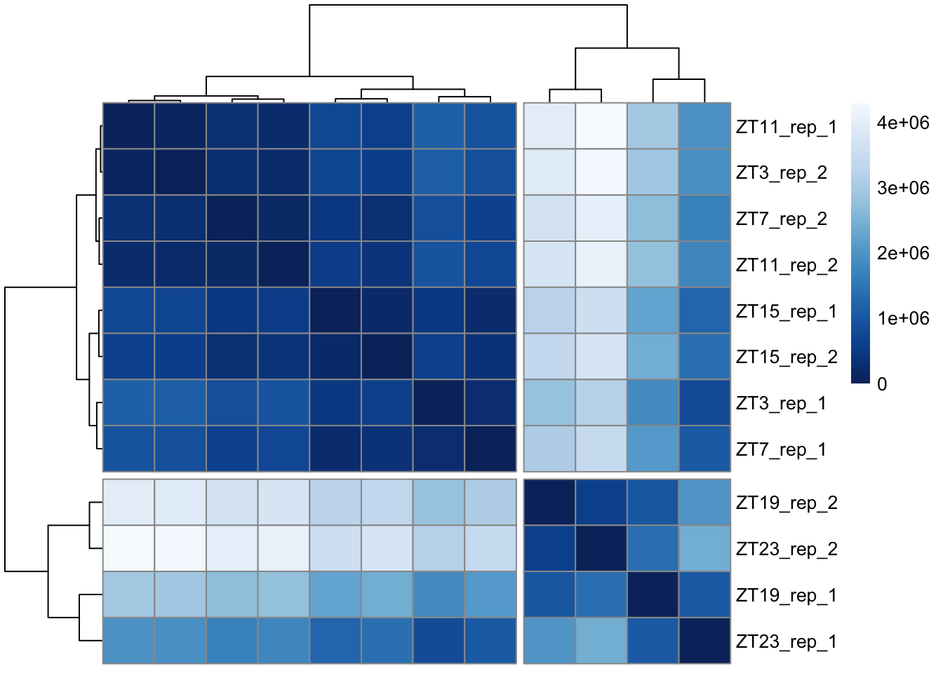

Figure 6.1: Heatmap representing distance between samples

PCA using DeSeq2

We have to do a logarithmic transformation to see how the data looks like after minimizing differences between samples for rows with small counts, and which normalizes with respect to library size. You can read the help executing ?rlog.

rdl.DN1 <- rlog(dds.DN1) 

Now we can plot the PCA analysis already integrated in the DeSeq2 package.

plotPCA(rdl.DN1, intgroup=c("ZT"))

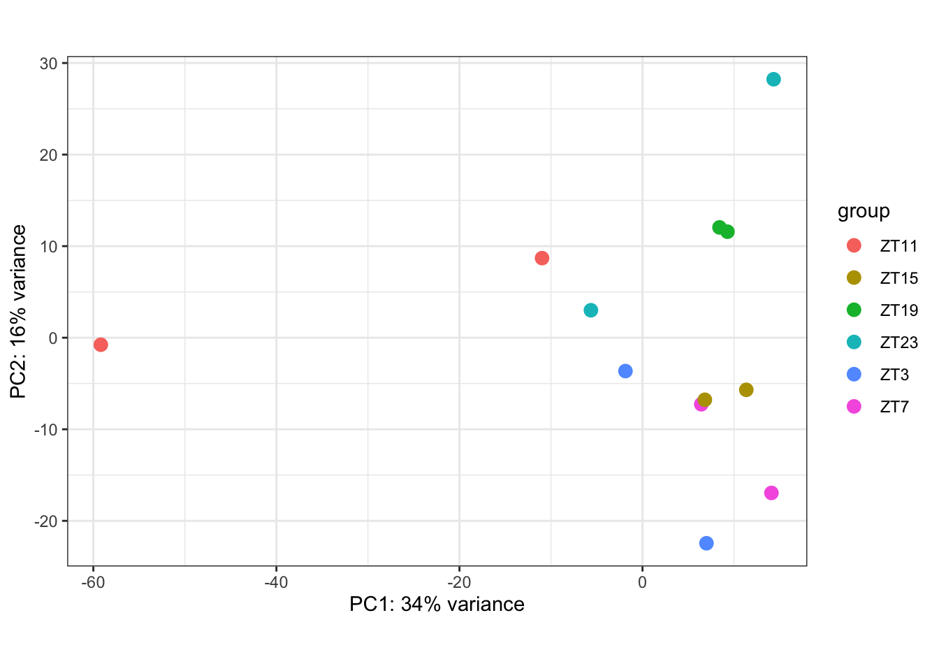
Figure 6.2: PCA coloring by ZT

PCA using basic R

We will use the function prcomp() to calculate the PCs. But before we do that we will select the most variable genes across samples. If a gene has the same value across all the samples will not be explicative or informative.

rv <- rowVars(assay(rdl.DN1)) # we calcualte the total variation in each gene (in this case rows), rowwVars literally calculates the variance in the rows
ntop <- 10000 # we select how many gene we want to use 
sg <- order(rv, decreasing = TRUE)[seq_len(min(ntop, length(rv)))] # here we select the most variable genes acording to the ntop value we set up before
mat <- t(assay(rdl.DN1)[sg, ]) # here we extract then the counts using the function assay from DeSeq2
pc <- prcomp(mat) # calcualte PCs
#head(pc,n=3L)

To select how many PCs are “important” we will use the percentage of variance explained by each PC. This takes us to the next step of understanding PCA. Each PC might be seen as a vector that explain some part of the variation of the data. Then if a PC explains only 2% of the data it makes no sense to pay attention to if we compared it to other PCs that might explain more.

fviz_eig(pc, addlabels = TRUE)

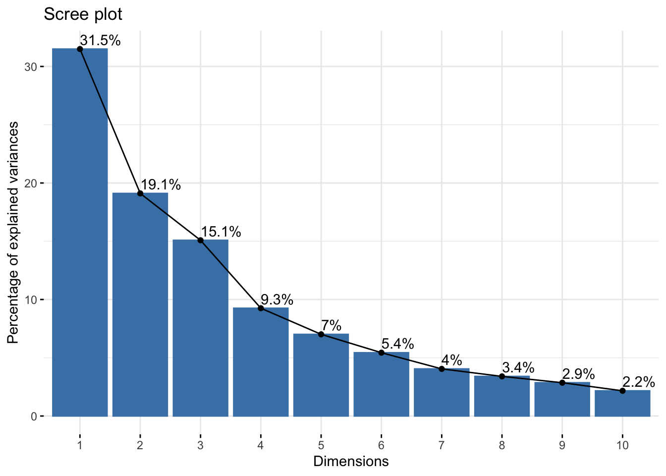
Figure 5.3: Variance explained by each PC

Now we can plot more than 2 PCs

pc_df=as.data.frame(pc$x) #transform to data frame
pc_df=merge(pc_df,colData.DN1,by="row.names",all=T) # merge with the colData to have the meta data of each saple
rownames(pc_df)=pc_df$Row.names


p1=ggplot(pc_df, aes(PC1, PC2, color=ZT)) +
  geom_point(size=3)  +
  theme_minimal()


p2=ggplot(pc_df, aes(PC3, PC2, color=ZT)) +
  geom_point(size=3) +
  theme_minimal()

#and both together
grid.arrange(p1,p2, ncol=2)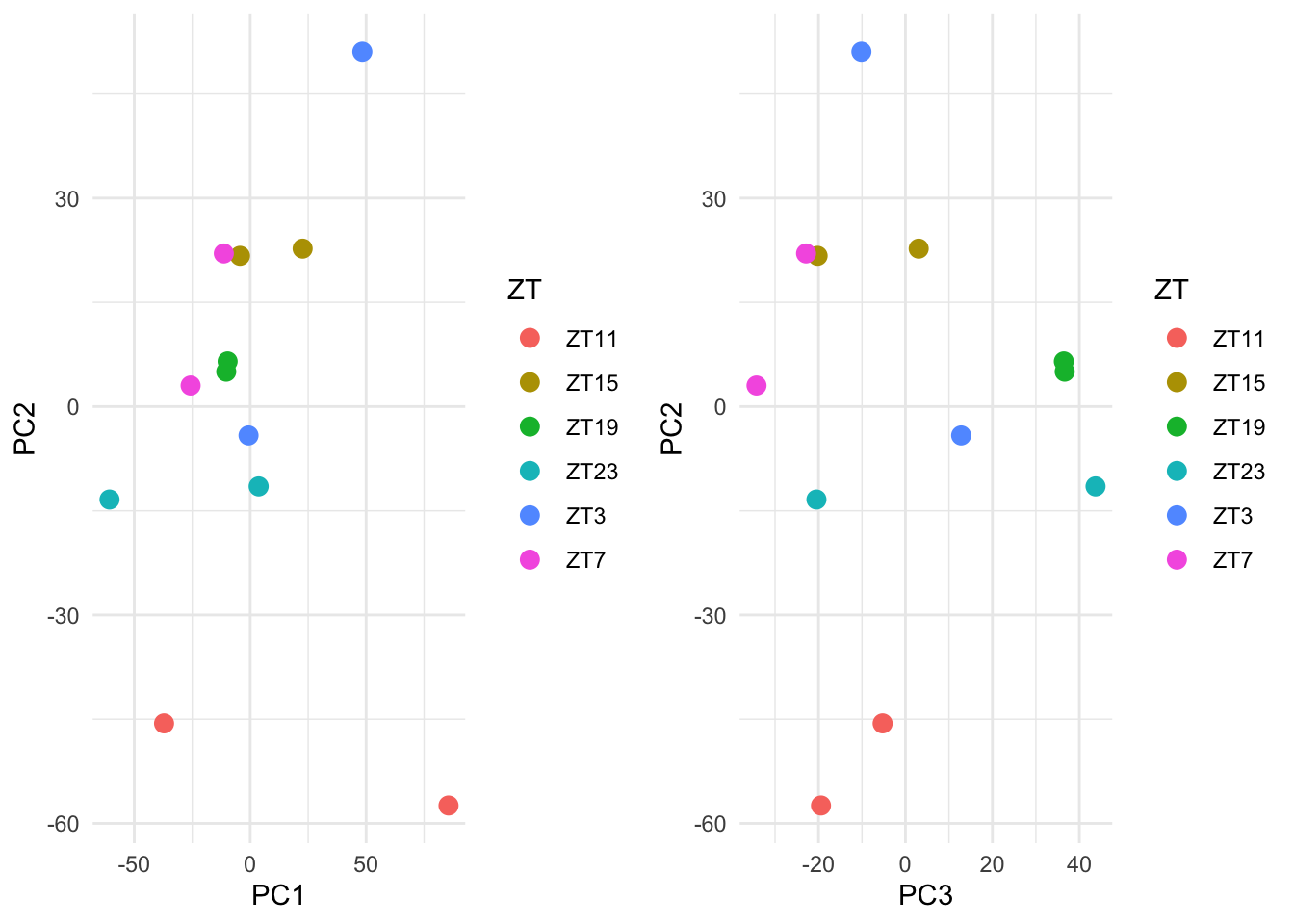

Figure 5.4: Ploting many principal components

p1=ggplot(pc_df, aes(PC1, PC2, color=ZT,label=Row.names)) +
  geom_point(size=3) +
  geom_label_repel(aes(label = Row.names),
                   box.padding   = 0.35, 
                   point.padding = 0.5,
                   segment.color = 'grey50') +
  theme_minimal()


p2=ggplot(pc_df, aes(PC3, PC2, color=ZT,label=Row.names)) +
  geom_point(size=3) +
  geom_label_repel(aes(label = Row.names),
                   box.padding   = 0.35, 
                   point.padding = 0.5,
                   segment.color = 'grey50') +
  theme_minimal()


#and both together
grid.arrange(p1,p2, ncol=2)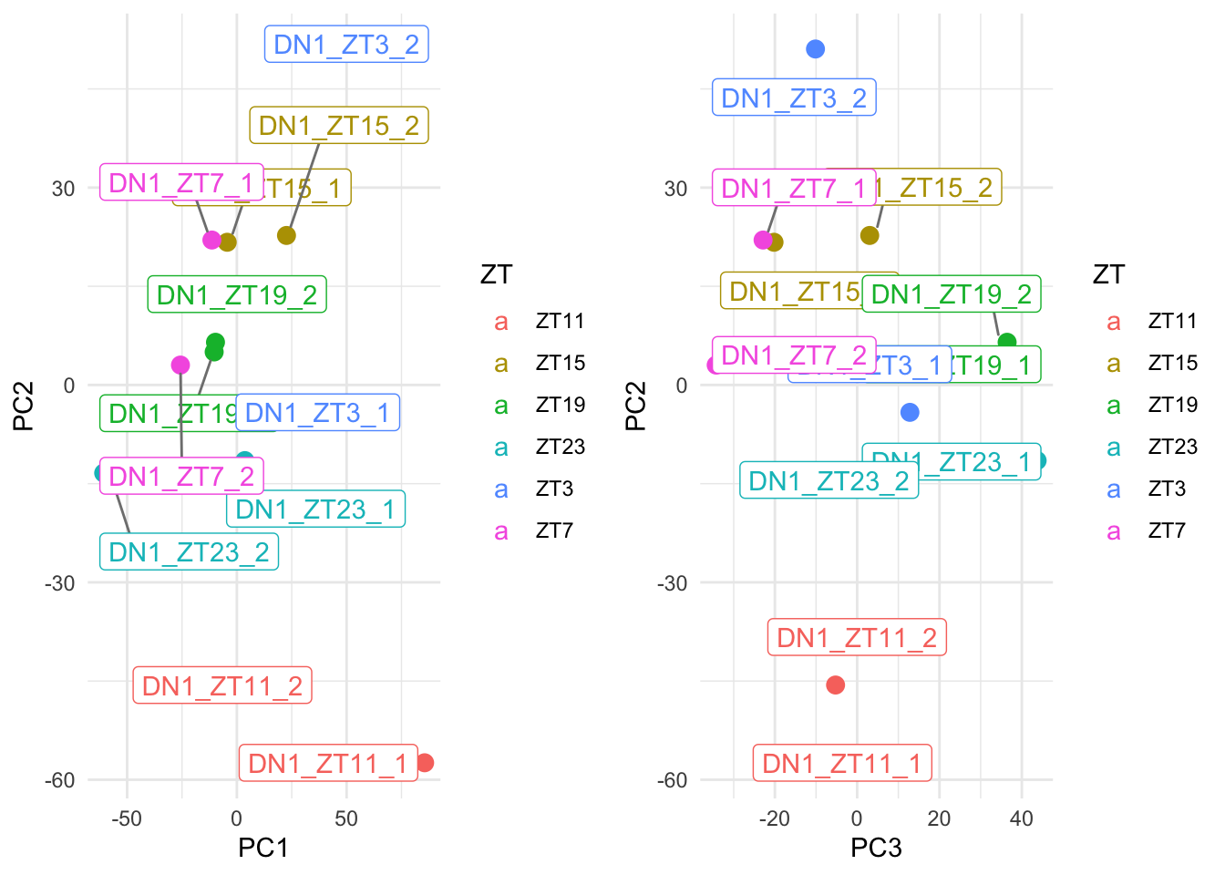

Figure 6.3: Ploting many principal components

#We can do some fancy 3D plots also, try them!
plot_ly(pc_df, x = ~PC1, y = ~PC2, z = ~PC3, color = ~ZT,colorscale = c('#FFE1A1', '#683531'))

plot_ly(pc_df, x = ~PC2, y = ~PC3, z = ~PC4, color = ~ZT,colorscale = c('#FFE1A1', '#683531'))

6.3.5 Differential gene expression analysis between ZT.

We already saw that for DN1: ZT19 and ZT23 looks more similar between them and also ZT3, 7, 15 and 11. We will now explore particular differences. DESeq is the main function here it acts over the object created previously. It executes the normalization and differential gene expression analysis.

Run differentially expression

dds.DN1 = DESeq(dds.DN1)

## estimating size factors

## estimating dispersions

## gene-wise dispersion estimates

## mean-dispersion relationship

## final dispersion estimates

## fitting model and testing

#The resultNames is taking the names of the comparisons done by the DESeq function
resultsNames(dds.DN1)

## [1] "Intercept"       "ZT_ZT15_vs_ZT11" "ZT_ZT19_vs_ZT11" "ZT_ZT23_vs_ZT11"
## [5] "ZT_ZT3_vs_ZT11"  "ZT_ZT7_vs_ZT11"

The results function extract this result, we will compare ZT3 vs ZT15. Use ?results to explore this function further.

res.ZT3vsZT15.DN1 <- results( dds.DN1, contrast = c("ZT","ZT3", "ZT15"),alpha=0.05)

head(res.ZT3vsZT15.DN1)

## log2 fold change (MLE): ZT ZT3 vs ZT15 
## Wald test p-value: ZT ZT3 vs ZT15 
## DataFrame with 6 rows and 6 columns
##                      baseMean log2FoldChange            lfcSE      stat
##                     <numeric>      <numeric>        <numeric> <numeric>
## FBtr0070202                 0             NA               NA        NA
## FBtr0070207   2.1168359707544              0 5.24448449612991         0
## FBtr0070238  2.68357323289241              0  4.8861753047644         0
## FBtr0070251 0.304433817751997              0 5.39799191011387         0
## FBtr0070484 0.151419583982656              0 5.39799191011387         0
## FBtr0070489                 0             NA               NA        NA
##                pvalue      padj
##             <numeric> <numeric>
## FBtr0070202        NA        NA
## FBtr0070207         1         1
## FBtr0070238         1         1
## FBtr0070251         1        NA
## FBtr0070484         1        NA
## FBtr0070489        NA        NA

What do you think is each column?

mcols(res.ZT3vsZT15.DN1)$description

## [1] "mean of normalized counts for all samples"
## [2] "log2 fold change (MLE): ZT ZT3 vs ZT15"   
## [3] "standard error: ZT ZT3 vs ZT15"           
## [4] "Wald statistic: ZT ZT3 vs ZT15"           
## [5] "Wald test p-value: ZT ZT3 vs ZT15"        
## [6] "BH adjusted p-values"

We can see the distribution of each variable using the function summary

summary(res.ZT3vsZT15.DN1)

## 
## out of 25337 with nonzero total read count
## adjusted p-value < 0.05
## LFC > 0 (up)       : 79, 0.31%
## LFC < 0 (down)     : 55, 0.22%
## outliers [1]       : 0, 0%
## low counts [2]     : 3419, 13%
## (mean count < 2)
## [1] see 'cooksCutoff' argument of ?results
## [2] see 'independentFiltering' argument of ?results

Identify differentially expressed genes: Multiple comparison correction and adjusted pvalue

You might have noticed that apart from pvalues there are adjusted pvalues. Just to recap, when we want to make conclusion we always have some chance to make a mistake. This chance increase with each element we add to out conclusions. Image what happens when we want to make a conclusion about 10.000 genes! We then correct the pvalue. There are different methods, in this case DeSeq2 uses Benjamini-Hochberg adjusted P value.

We can now do an histogram to explore how is the distribution of the padj.

#histogram
hist(res.ZT3vsZT15.DN1$padj, breaks=100, col="skyblue", border="slateblue", main="")

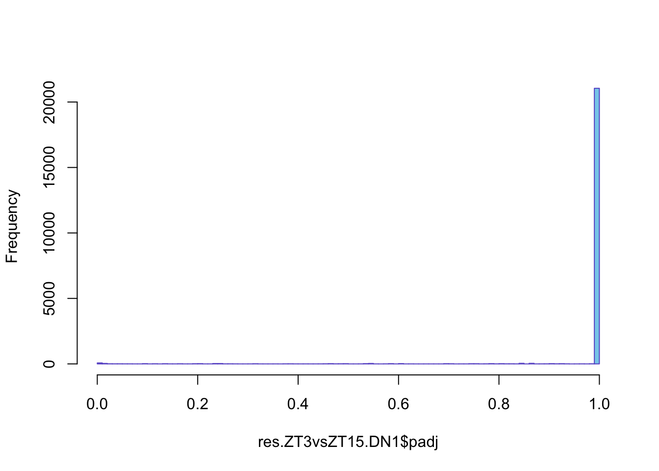
Figure 6.4: Histogram of pjusted value distribution

Identify differentially expressed genes: Log2(FoldChange)

Identify differentially expressed genes is a combination of pvalue and a fold change. Fold change is literally the comparison of 2 conditions. Let’s go back to our example.

Row Names	WildType.1	WildType.2	Mutant.1	Mutant.2
geneA	230	210	420	412

Here, geneA seems to be around 2 times more in Mutant compared with the WildType. This would be an UPregulated gene.

\[ Mutant/WT=400/200=2 \]

If we imagine the opposite situation, a DOWNregulated gene, the same comparison would give a not-such intuitive result.

Row Names	WildType.1	WildType.2	Mutant.1	Mutant.2
geneA	430	410	220	212

\[ Mutant/WT=200/400=0.5 \]

To avoid this, in differential gene expression we use log2. This will give us the following:

\[ UPregulated: log2(Mutant/WT)=log2(400/200)=1 \] \[ DOWNregulated: log2(Mutant/WT)=log2(200/400)=-1 \]

To know what is being used as denominator (control) we can look into the DeSeq2 manual: “With no additional arguments to results(), the log2 fold change and Wald test p value will be for the last variable in the design formula, and if this is a factor, the comparison will be the last level of this variable over the reference level.”

In our case then ZT15 is being used as reference

To see significance is to use MA plots which shows log2 fold changes (on the y-axis) versus the mean of normalized counts (on the x-axis).

plotMA(res.ZT3vsZT15.DN1,alpha=0.05) #In red everything with padj < 0.05

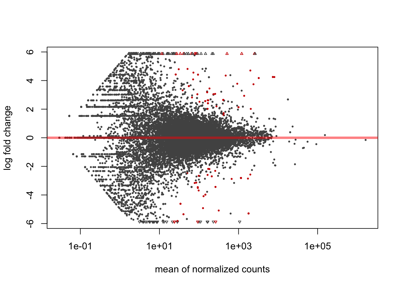
Figure 6.5: MA plot: log2 fold changes vs normalized counts

6.3.6 Explore results

We can create a data frame of the results and play around.

res.ZT3vsZT15.DN1_df<-as.data.frame(res.ZT3vsZT15.DN1)
res.ZT3vsZT15.DN1_df=res.ZT3vsZT15.DN1_df[complete.cases(res.ZT3vsZT15.DN1_df),]#remove NAs
res.ZT3vsZT15.DN1_df$transcript_name=rownames(res.ZT3vsZT15.DN1_df)

head(res.ZT3vsZT15.DN1_df)

##              baseMean log2FoldChange     lfcSE      stat     pvalue padj
## FBtr0070207  2.116836      0.0000000 5.2444845  0.000000 1.00000000    1
## FBtr0070238  2.683573      0.0000000 4.8861753  0.000000 1.00000000    1
## FBtr0070658  2.762362      0.0000000 5.3979919  0.000000 1.00000000    1
## FBtr0071170 16.483738      2.1943705 1.1682234  1.878383 0.06032885    1
## FBtr0071173  4.674766      0.0000000 5.3502754  0.000000 1.00000000    1
## FBtr0071619 49.515374     -0.8457701 0.6368886 -1.327972 0.18418743    1
##             transcript_name
## FBtr0070207     FBtr0070207
## FBtr0070238     FBtr0070238
## FBtr0070658     FBtr0070658
## FBtr0071170     FBtr0071170
## FBtr0071173     FBtr0071173
## FBtr0071619     FBtr0071619

Change the gene names

As you can see, the names of the genes are in a nomenclature that is not intuitive. We can then use some functions that will allow us to change the names for some more informative.

Let’s take one example: FBtr0070207, is a transcript name (not a gene name, but one of the possible variants of the gene) http://flybase.org/reports/FBtr0070207. We want for this analysis the gene name. For that we will use the package org.Dm.eg.db (each model organism has one of this: https://bioconductor.org/packages/release/BiocViews.html#___AnnotationData)

#Explore the options that the package gives us
keytypes(org.Dm.eg.db)

##  [1] "ACCNUM"       "ALIAS"        "ENSEMBL"      "ENSEMBLPROT"  "ENSEMBLTRANS"
##  [6] "ENTREZID"     "ENZYME"       "EVIDENCE"     "EVIDENCEALL"  "FLYBASE"     
## [11] "FLYBASECG"    "FLYBASEPROT"  "GENENAME"     "GO"           "GOALL"       
## [16] "MAP"          "ONTOLOGY"     "ONTOLOGYALL"  "PATH"         "PMID"        
## [21] "REFSEQ"       "SYMBOL"       "UNIGENE"      "UNIPROT"

#We have here the ENSEMBLE transcript names, so we will use that keytype
genenames <- mapIds(org.Dm.eg.db,keys = rownames(dds.DN1),column = "SYMBOL",keytype="ENSEMBLTRANS")
annotation_DN1 <- data.frame(gene_name = genenames, transcript_name=rownames(dds.DN1), row.names = rownames(dds.DN1), stringsAsFactors = FALSE)
head(annotation_DN1) 

##             gene_name transcript_name
## FBtr0070202   CG14625     FBtr0070202
## FBtr0070207    fs(1)N     FBtr0070207
## FBtr0070238   CG11409     FBtr0070238
## FBtr0070251   CG11384     FBtr0070251
## FBtr0070484   fs(1)Yb     FBtr0070484
## FBtr0070489   CG12498     FBtr0070489

Now that we have a “mapping” we can use it. We will use the function merge.

res.ZT3vsZT15.DN1_df=merge(res.ZT3vsZT15.DN1_df,annotation_DN1,by="transcript_name")
head(res.ZT3vsZT15.DN1_df)

##   transcript_name  baseMean log2FoldChange     lfcSE       stat    pvalue padj
## 1     FBtr0005088 404.52656     -0.3962867 0.4939109 -0.8023445 0.4223537    1
## 2     FBtr0005673   2.35263      1.7199349 2.8262384  0.6085598 0.5428163    1
## 3     FBtr0005674   2.35263      1.7199349 2.8262384  0.6085598 0.5428163    1
## 4     FBtr0070000  44.02153     -0.7589507 1.1324434 -0.6701886 0.5027375    1
## 5     FBtr0070002   4.30420      3.7116759 2.5555706  1.4523863 0.1463942    1
## 6     FBtr0070006  23.06487     -1.1075368 1.0502903 -1.0545054 0.2916516    1
##   gene_name
## 1  Pp2A-29B
## 2      <NA>
## 3      <NA>
## 4      Nep3
## 5    CG9570
## 6    CG9572

UP regulated genes Now let’s look for the genes that are changing with than Log2foldChange > 1 (which is a fold change of 2)

sig_down=unique(res.ZT3vsZT15.DN1_df$gene_name[(res.ZT3vsZT15.DN1_df$padj<0.05&res.ZT3vsZT15.DN1_df$log2FoldChange<(-1))])
head(sig_down)

## [1] NA        "CG14089" "CG13041" "CG32137" "Pdp1"    "tim"

DOWN regualted genes Now let’s look for the genes that are changing with than Log2foldChange < -1 (which is a fold change of 0.5, so a downregulation of 2 times)

sig_up=unique(res.ZT3vsZT15.DN1_df$gene_name[(res.ZT3vsZT15.DN1_df$padj<0.05&res.ZT3vsZT15.DN1_df$log2FoldChange>1)])

head(sig_down)

## [1] NA        "CG14089" "CG13041" "CG32137" "Pdp1"    "tim"

Plot genes

Let’s plot some genes using DeSeq2.

plotCounts(dds.DN1, gene=which.min(res.ZT3vsZT15.DN1$padj), intgroup="ZT")

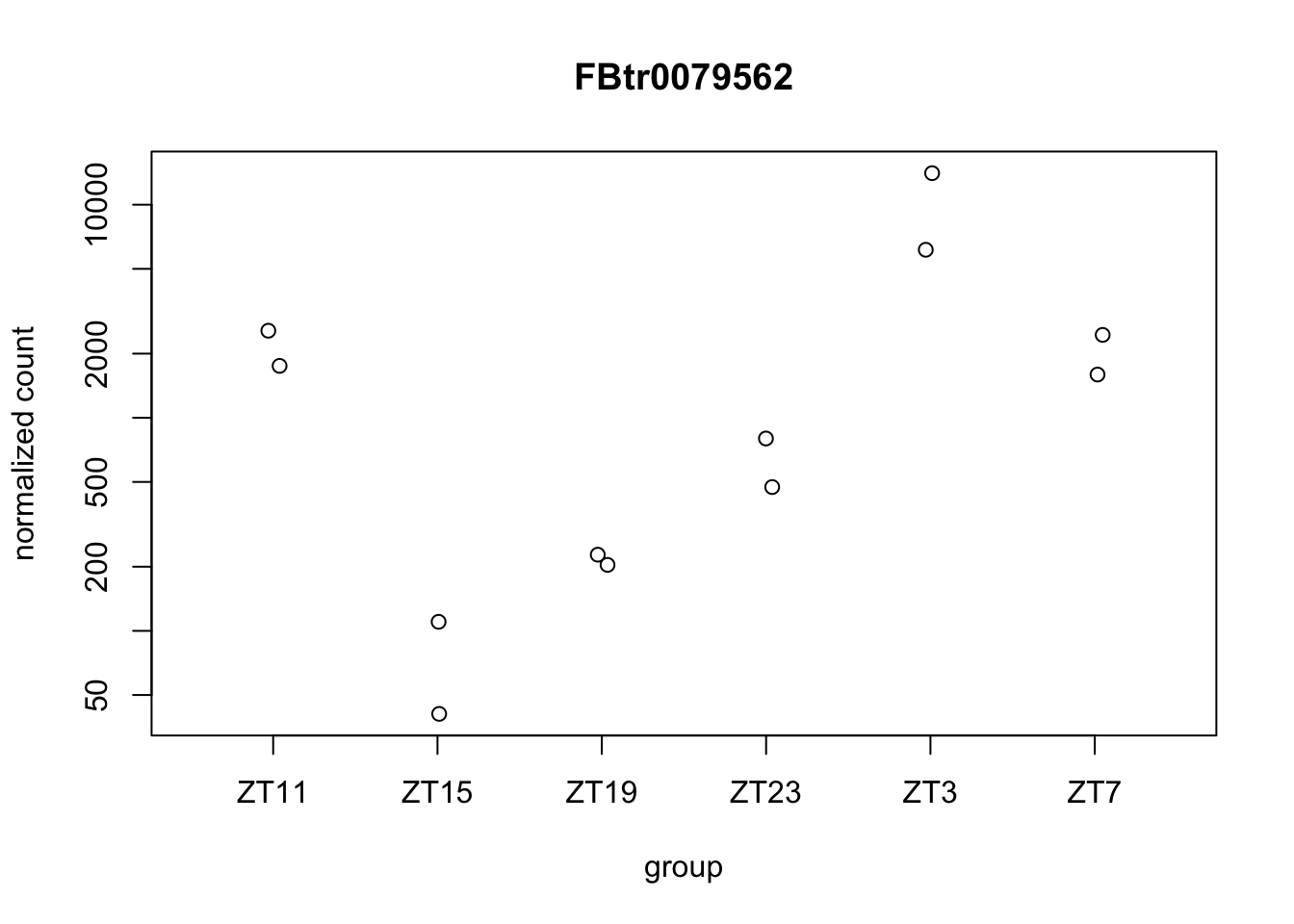
Figure 6.6: Plot gene expression.

plotCounts(dds.DN1, gene="FBtr0077567", intgroup="ZT")

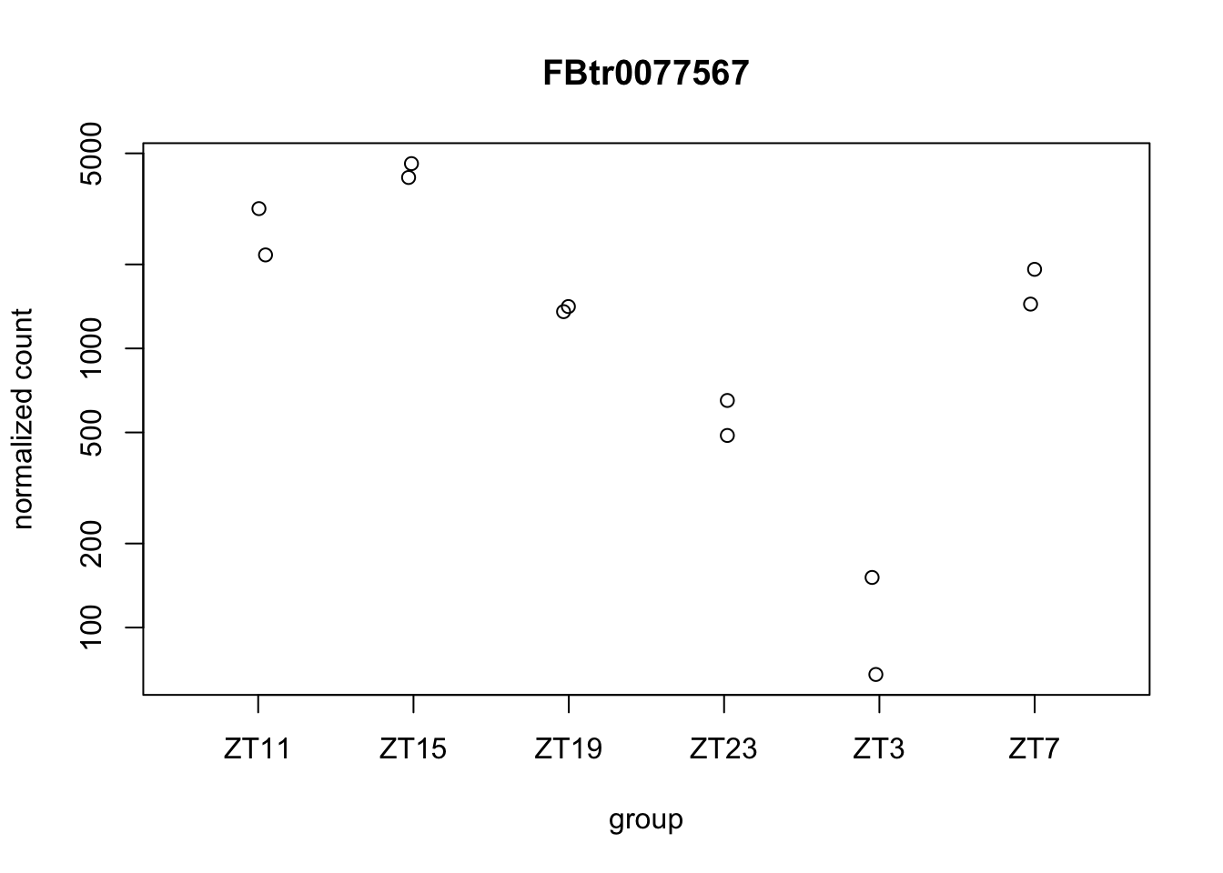
Figure 6.7: Plot gene expression.

We can do this in ggplot2

d <- plotCounts(dds.DN1, gene="FBtr0077567", intgroup="ZT", returnData=TRUE) #extract eh data from the plot

ggplot(d, aes(x=ZT, y=count)) + geom_point(position=position_jitter(w=0.1,h=0)) #use it to plot in a better way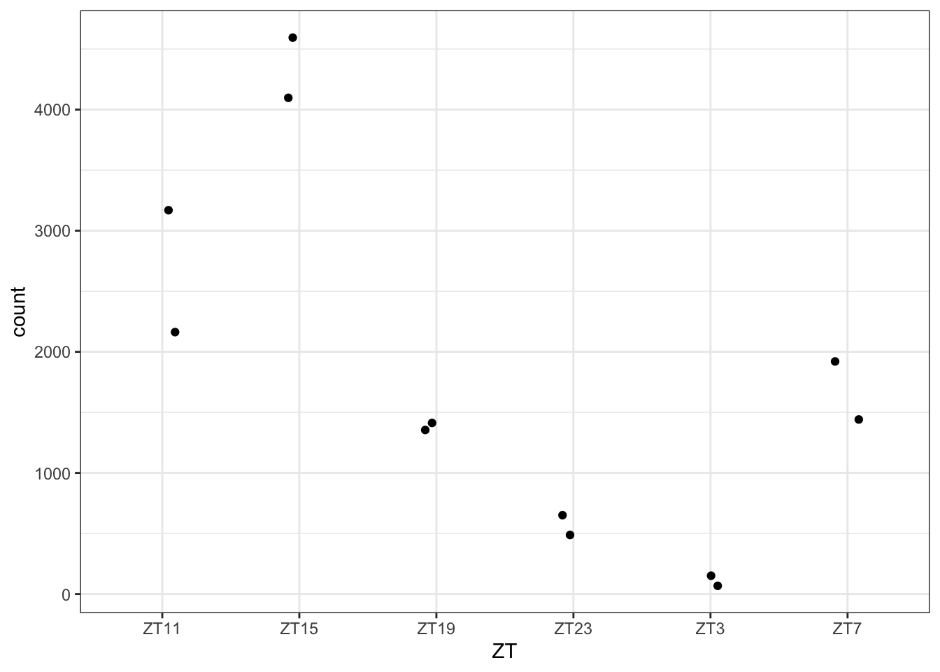

Figure 3.11: Plot gene expression using ggplot.

Let’s discuss what we see in the graphics.

We have some of the figures that seems to have the exactly same values for each replicate. This is at least suspicious. This might be just the same quantification so it might not be correct to say that they are different isoforms and maybe it is better to collapse them or change the strategy to analyze different isoforms. This also shows us the limitations we have when we use the data already aligned.

6.3.7 Plot counts using ggplot

Let’s see how we can plot the transcript reads in a better way. Doing a few manipulations on the table we can have even better plots.

#big plot
#I take the normalized values and do the plots
toplot<-as.data.frame(as.data.frame(counts(dds.DN1, normalized=T)))
toplot$transcript_name<-rownames(toplot)

toplot<-toplot %>% gather(zt_rep, value, -transcript_name) #This is a more complex line of code, let’s explore the results.
head(toplot)

##   transcript_name    zt_rep value
## 1     FBtr0070202 DN1_ZT3_1     0
## 2     FBtr0070207 DN1_ZT3_1     0
## 3     FBtr0070238 DN1_ZT3_1     0
## 4     FBtr0070251 DN1_ZT3_1     0
## 5     FBtr0070484 DN1_ZT3_1     0
## 6     FBtr0070489 DN1_ZT3_1     0

toplot=merge(toplot,annotation_DN1,by="transcript_name")
head(toplot)

##   transcript_name     zt_rep    value gene_name
## 1     FBtr0005088 DN1_ZT11_2 333.0941  Pp2A-29B
## 2     FBtr0005088 DN1_ZT19_2 332.2765  Pp2A-29B
## 3     FBtr0005088  DN1_ZT7_2 520.4211  Pp2A-29B
## 4     FBtr0005088  DN1_ZT3_2 235.0216  Pp2A-29B
## 5     FBtr0005088 DN1_ZT23_2 392.4796  Pp2A-29B
## 6     FBtr0005088 DN1_ZT19_1 406.2523  Pp2A-29B

What changed here? How this allow for better plotting?

#Lets create now more meta data 
toplot$zt<-sapply(strsplit(as.character(toplot$zt_rep),"_"),"[[",2)
toplot$ztime<-gsub(toplot$zt,pattern = "ZT",replacement = "")
toplot$rep<-sapply(strsplit(as.character(toplot$zt_rep),"_"),"[[",3)
toplot$ztime_2<-as.numeric(toplot$ztime)
toplot$ztime_2[toplot$rep=="2"]<-toplot$ztime_2[toplot$rep=="2"]+24

#And plot
genes.cyc = c("tim","Clk","per","cwo") #you can put here as many genes as you want

ggplot(toplot[toplot$gene_name %in% genes.cyc ,],aes(x = as.numeric(ztime),y = value,color=gene_name,shape=rep)) + geom_point() + geom_line()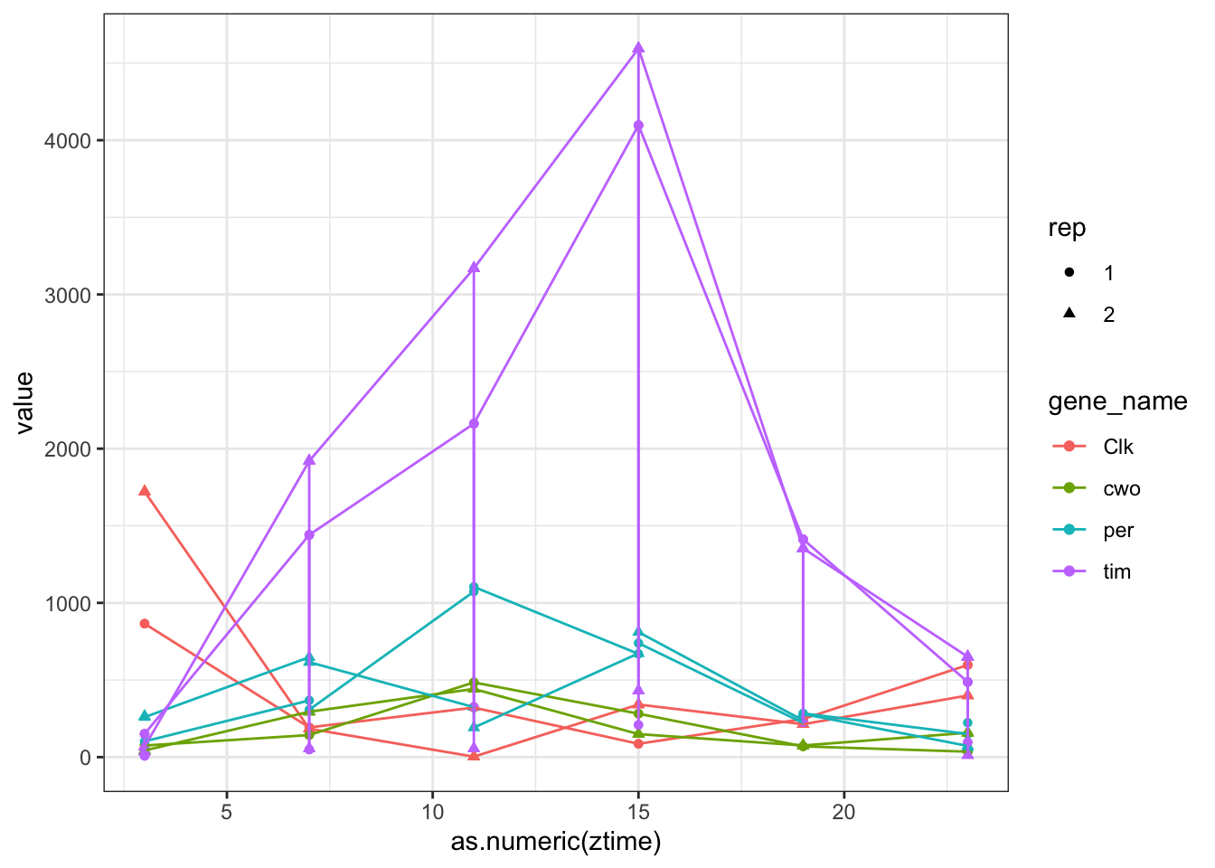 

Figure 6.8: Count plots with ggplot

ggplot(toplot[toplot$gene_name %in% genes.cyc ,],aes(x =ztime_2,y = value,color=gene_name,shape=rep)) + geom_point() + geom_line()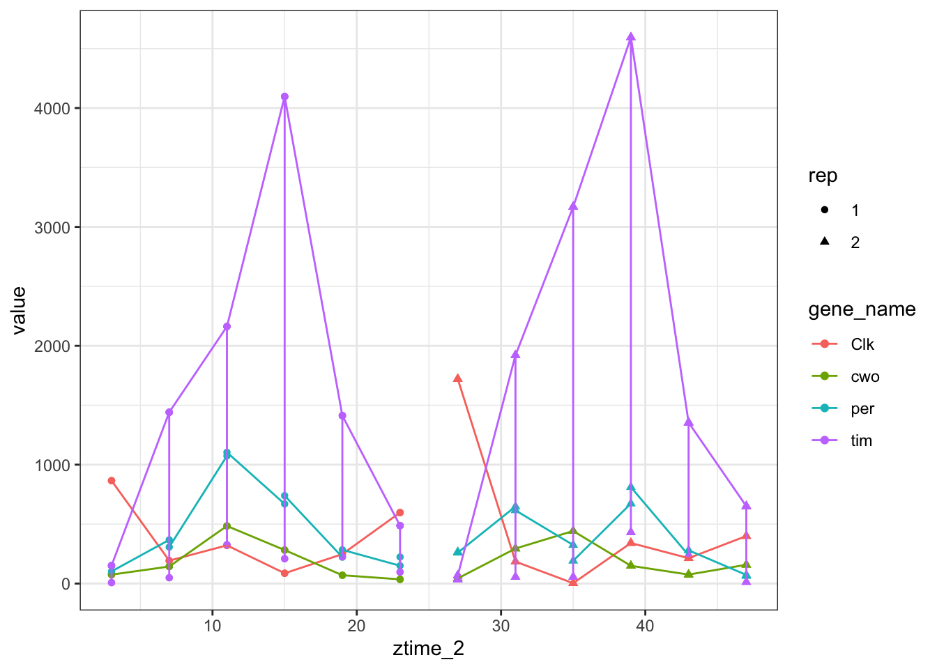

Figure 6.9: Count plots with ggplot using zt time

ggplot(toplot[toplot$gene_name %in% genes.cyc ,],aes(x =ztime_2,y = value,color=gene_name,shape=rep)) + geom_point() + geom_line() + facet_wrap(scales = "free",facets = ~gene_name )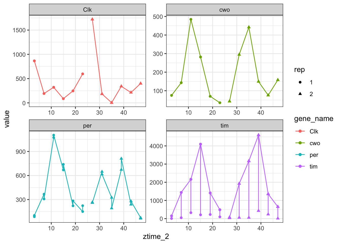

Figure 3.16: Count plots with ggplot sepparating by gene name

6.4 Gene Ontology (GO) term analysis

The main objective of GO term analysis is to identify common features in a list of gene shared feature that might be “enriched” when compared with the background list of of genes. There are 3 GO term sets:

1. Molecular Function(MF): Molecular function or activities performed by gene product. Examples can be for example catalysis or transport.
2. Biological Process(BP): The larger processes, or ‘biological programs’ that these genes takes part in. Examples can be DNA repair or signal transduction.
3. Cellular Component(CC): The locations relative to cellular structures in which a gene product performs a function, either cellular compartments.

For this we use the known information about each gene. Lets see one example: Gad1.

From FlyBase: “Glutamic acid decarboxylase 1 (Gad1) encodes an essential, nervous system-specific glutamic acid decarboxylase, which is the synthetic enzyme for the major inhibitory neurotransmitter gamma-Aminobutyric acid (GABA). It is required for a multitude of physiological functions and adult behaviors dependent on GABA, including sleep, memory, circadian rhythms and egg hatching.”

Then, MF GO term are glutamate decarboxylase activity, glutamate decarboxylase activity, pyridoxal phosphate binding. BP: gamma-aminobutyric acid biosynthetic process,glutamate catabolic process,larval locomotor behavior,neuromuscular junction development,neurotransmitter receptor metabolic process,olfactory learning CC: cytosol

Basically then, if a term appears more than “by chance” in a gene list, it will be then significantly enriched.

There are many online tools to do this type of analysis (http://cbl-gorilla.cs.technion.ac.il/, ) but here we will use the R package topGO.

We will analyze the results from the RNA seq. It is important to know what to use as a background list of genes. In this case, any expressed gene in the cell-type we are analyzing.

topGO requires a list of genes with an indicator of 1 for the genes that should be taken into the analysis and the rest with 0. The full list of genes will be used as background.

To get the list of expressed genes we will use the fact that DeSeq2 actually puts NA in the padjusted column to the lowly expressed genes.

#Libraries
library("topGO")
library("org.Dm.eg.db")

#Prepare list of genes that are expressed, complete cases will get rid of the genes with NAs
genes<-as.data.frame(res.ZT3vsZT15.DN1_df$gene_name[complete.cases(res.ZT3vsZT15.DN1_df)])
names(genes)<-"gene_name"

#Add the indicator
genes$ind=0
genes$ind[genes$gene_name %in% sig_up] = 1

alg <- factor( as.integer( genes$ind ) )
names(alg) <- genes$gene_name
onts = c( "MF", "BP", "CC" )

tab = as.list(onts)
listGOtab =  as.list(onts)
names(tab) = onts

#For loop going over the 3 GO term sets
for(e in 1:3){
  
  #start topGO data
  tgd <- new( "topGOdata", ontology=onts[e], allGenes = alg, nodeSize=5,
              annot=annFUN.org, mapping="org.Dm.eg.db", ID = "symbol" )
  listGO = genesInTerm(tgd)
  
  resultTopGO.elim <- runTest(tgd, algorithm = "elim", statistic = "Fisher" )
  resultTopGO.classic <- runTest(tgd, algorithm = "classic", statistic = "Fisher" )
  tab[[e]] <- GenTable( tgd, Fisher.elim = resultTopGO.elim, 
                        Fisher.classic = resultTopGO.classic,
                        orderBy = "Fisher.classic",  topNodes =  100)
  tab[[e]]$FDR<-p.adjust(tab[[e]]$Fisher.classic,method = "fdr") #I correct the pvalues 
  tab[[e]]$ontology=onts[e]
}

allGO = rbind (as.data.frame(tab[[2]]),as.data.frame(tab[[1]]),as.data.frame(tab[[3]]))
write.table(allGO, paste0("GOterm.txt"),sep = "\t" , row.names=F)

6.5 Extra: negative binomial model

The model would be then: counts Kij for gene i, sample j are modeled using a negative binomial distribution with fitted mean μij and a gene-specific dispersion parameter αi. The fitted mean is composed of a sample-specific size factor sj and a parameter qij proportional to the expected true concentration of fragments for sample j.

\[ K_{ij}∼NB(μ_{ij},α_i) \] \[ μij=s_jq_{ij} \]

6.6 Activity

Finish the analysis for the other cell-types. Find a way to compare the results (hint: look at dendrograms)

6.7 Resources and Bibliography

Dubowy C, Sehgal A. Circadian Rhythms and Sleep in Drosophila melanogaster. Genetics. 2017;205(4):1373-1397. doi:10.1534/genetics.115.185157

MEIRELES-FILHO, Antonio Carlos Alves and KYRIACOU, Charalambos Panayiotis. Circadian rhythms in insect disease vectors. Mem. Inst. Oswaldo Cruz [online]. 2013, vol.108, suppl.1 [cited 2020-07-08], pp.48-58.

Abruzzi KC, Zadina A, Luo W, Wiyanto E, Rahman R, Guo F, et al. (2017) RNA-seq analysis of Drosophila clock and non-clock neurons reveals neuron-specific cycling and novel candidate neuropeptides. PLoS Genet 13(2): e1006613. https://doi.org/10.1371/journal.pgen.1006613

Schubert FK, Hagedorn N, Yoshii T, Helfrich-Förster C, Rieger D. Neuroanatomical details of the lateral neurons of Drosophila melanogaster support their functional role in the circadian system. J Comp Neurol. 2018;526(7):1209-1231. doi:10.1002/cne.24406

DeSeq2 documentations: http://bioconductor.org/packages/release/bioc/vignettes/DESeq2/inst/doc/DESeq2.html

Introduction to implementation steps of MetaCycle Gang Wu, Ron Anafi, Michael Hughes, Karl Kornacker, and John Hogenesch 2015-12-04 https://cran.r-project.org/web/packages/MetaCycle/vignettes/implementation.html

Gene Ontology overview http://geneontology.org/docs/ontology-documentation/