Lab 5 Chip Sequencing Analysis
5.1 Objectives
After this section you should be able to:
- Explore results from ChipSeq data.
- Modify tables and change gene names.
- Use different ChipSeq gene annotation packages from R.
- Find sequence motif enrichment in sequencing data.
5.2 Introduction
Chip-seq procedure:
“ChIP-seq” is short for “chromatin immunoprecipitation (ChIP) followed by sequencing (seq)”. ChipSeq data is basically DNA sequencing data in which the DNA is sequenced AFTER immunoprecipitating a protein of interest. Therefore, we expect to sequence the pieces of DNA that are interacting with the precipitated protein.
If the protein of interest is a transcription factor (TF) for example, we expect to get the regions of DNA close to the genes that are being regulated by this particular TF (ie. the promoters of the genes). If we immunoprecipitate RNA polymerase 2, we expect to get the regions of the DNA that are being transcribed to RNA.
But, how do we know if certain region of the genome is really interreacting with the protein of interest? As in any analysis, it is important to have a control to see the probability to have a signal in a particular region just by chance. Usually as a control we use the DNA sequencing BEFORE immunoprecipitation (IP). This data is usually called input (INP), as it is the input material used for the IP. What we are looking then will be “enrichment” of each region of the genome in the IP compared with the INP.
The biochemical procedure usually goes as follows:
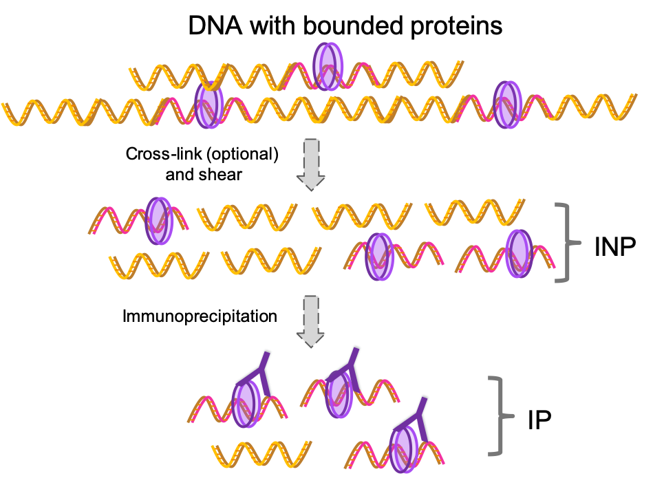
Figure 1.1: Commonly used ChipSeq procedure. DNA is fragmented followed by immunoprecipitation for the protein of interest. Finally, DNA library is prepared and sequenced. As you can see there is an enrichment of the DNA regions bonded to the protein of interest.
To study this type of data we will re-analyze the data generated in Meireles-Filho et al 2014.
In this work the authors study genome-wide the binding of two transcription factors (Clk and Cyc) in the fruit fly (Drosophila melanogaster). To do so they do Chip sequencing.
These two transcription factors are core components of the circadian clock in animals. Just as an introduction these two transcription factors bind to specific regions on the genome and activate transcription. Clk oscilates over the day due to a set of feedback loops with other core-clock components. These set of molecular interactions generate an autonomous oscilating molecular clock with a period of almost 24 hr. This clock can be re-set by light input. We will study RNA oscilations over the day in next chapter.
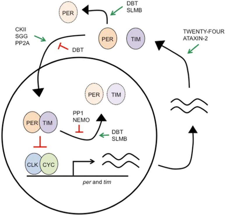
Figure 4.1: Circadian clock at the molecular level. The molecular feedback loop is formed by the negative feedback of Period (PER) and Timeless (TIM) on their own transcription. Figure adapted from Dubowy et al 2017
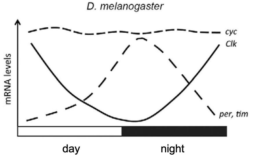
Figure 4.2: Cyc, Clk and Time levels over the day. Figure adapted from Alves Meireles-Filho et al 2013

Figure 4.3: Light control of the circadian clock. Figure adapted from Alves Meireles-Filho et al 2013
5.3 Data pre-processing (peak-calling):
Our goal is then to quantify signal enrichment in certain part of the genome in IP vs INP sequencing. This is achieved by comparing the ALIGNEMENT of the reads of IP vs INP.
This process is called “peak calling” because it is trying to determine the “pileup” of reads along the genome forming “peaks”. As any peak the algorithm used will report high of the peak, summit location, width and finally a pvalue corresponding to the comparison of the signal in that region in IP vs INP.
Here we can see how the pileup reads look like in IGV. We are looking here at the promoter of the genes tim, a known target of CLK protein. As you can see, the peak is clear in the IP comapred with the INP.
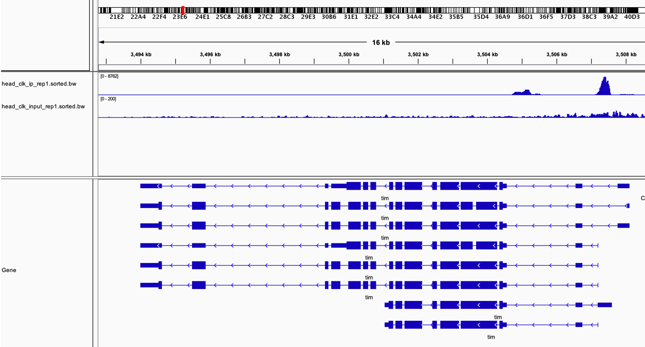
Figure 4.4: IGV pileup traks over tim. Upper line IP, lower line INP.
To do this analysis genome wide, we need a tool that can do this for all the genom. There are few tools available, we use here MACS algorithm to assess the peaks from the sequencing data.
Basically, this analysis relies in the aligned data (.bam files). It compares the IP with the INP control.
For this analysis I aligned the data from GEO with Bowtie2, an aligner that is used for DNA data (not splice aware).
Finally ran the MACS command in the terminal as follows:
macs2 callpeak -t head_clk_ip_rep1.sorted.bam head_clk_ip_rep2.sorted.bam -c ./head_clk_input_rep1.sorted.bam ./head_clk_input_rep2.sorted.bam -g dm -n PeakAna_clk_Ip_vs_INP -B -p 0.05Where, -t indicates that the following arguments are the IP samples, -c the control samples, -g the genome name in this case “dm”, -n the name that all the output files will have, -B indicates to the program to store visualization files (in .bdg format usefull to visualize in IGV).
The output after running MACS on the shell:
| File name | Description |
|---|---|
| PeakAna_clk_Ip_vs_INP_model.r | An R script for producing a PDF illustrating the peak model |
| PeakAna_clk_Ip_vs_INP_model.pdf | The PDF image of the read distribution in model peaks and fragment size estimation |
| PeakAna_clk_Ip_vs_INP_peaks.xls | Key parameters used by MACS and detailed information of every peak identified by MACS |
| PeakAna_clk_Ip_vs_INP_peaks.bed | Peak locations in BED format |
| PeakAna_clk_Ip_vs_INP_peaks.subpeaks.bed | Subpeak locations in BED-like format. This file is generated by PeakSplitter, which is called by MACS |
| PeakAna_clk_Ip_vs_INP_summits.bed | Summit locations of the peaks in BED format |
| PeakAna_clk_Ip_vs_INP_MACS_bedGraph | Directory where the BedGraph files are generated. For each control or ChIP-seq sample, a BedGraph file describes the read distribution along the whole genome |
5.4 Exploring the results:
We will see the first part of the output we get in the “NAME_peaks.xls”:
We can see here that we have all the columns we expect and we cqn try to see places we know are interesting for us.
#knitr::include_graphics('images/hex-rmarkdown.png')
macs.res<-read.table("../macs2_analysis_p0.05/PeakAna_clk_Ip_vs_INP_peaks_bed.txt",header = T)
head(macs.res)
## chr start end length abs_summit pileup X.log10.pvalue. fold_enrichment
## 1 chr2L 34224 34348 125 34306 20.88 2.75497 1.97319
## 2 chr2L 34965 35180 216 35108 23.26 3.33362 2.02190
## 3 chr2L 40369 40577 209 40492 30.42 7.01721 2.83398
## 4 chr2L 57282 57429 148 57365 22.07 3.47781 2.08079
## 5 chr2L 58368 58696 329 58541 39.37 12.02019 3.64098
## 6 chr2L 62014 62139 126 62048 19.68 2.42109 1.86559
## X.log10.qvalue. name
## 1 1.12350 PeakAna_clk_Ip_vs_INP_peak_1
## 2 1.65302 PeakAna_clk_Ip_vs_INP_peak_2
## 3 5.05903 PeakAna_clk_Ip_vs_INP_peak_3
## 4 1.77350 PeakAna_clk_Ip_vs_INP_peak_4
## 5 9.82848 PeakAna_clk_Ip_vs_INP_peak_5
## 6 0.83175 PeakAna_clk_Ip_vs_INP_peak_65.5 Annotating the peaks.
With this information we want to be able to conclude something about this transcription factor regulation.
The first thing to see is genes that might be regulated. This is basically looking which is the closest gene to each peak.
To do this we will just looking at the annotation file that have the information of which gene is in each region of the genome (we can think of this as the “map” of the genome).
What problems you can think that this approach might have? Think about enhancers for example.
For this we will use the following libraries:
library(GenomicFeatures) #This is an R package to deal with genomic data. You can read more at https://bioconductor.org/packages/release/bioc/vignettes/GenomicFeatures/inst/doc/GenomicFeatures.pdf
library(ChIPpeakAnno) #This is a package to annotate Chip-Peaks data https://bioconductor.org/packages/release/bioc/vignettes/ChIPpeakAnno/inst/doc/ChIPpeakAnno.html
5.5.1 Read the annotation file
In class we saw what were annotation files. Those were files that contained the “map” of the genome. This map shows us where each gene start and end and where each exon, intron and UTR is in that gene.
We will work with a GTF file. Remember that annotation files can be in many formats. They can be downloaded from different places as UCSC genome browser, Ensemble, etc.
To read the GTF file we will use the makeTxDbFromGFF function. We are doing this because it will allow us to change it to another format, sqlite.
txdb <- makeTxDbFromGFF(file="../macs2_analysis_p0.05/annot2.chr.gtf", format = "gtf", dataSource="dm6", organism="Drosophila melanogaster") #this funciton is actually reading the GTF file and creating a data base. Try reading the help documentation of this funciton.

#Now we need to save this as an sqlite:
saveDb(txdb, file="../macs2_analysis_p0.05/dm6.sqlite") #Look at your working directory, what happened?
txdb <- loadDb("../macs2_analysis_p0.05/dm6.sqlite") #this is loading the sqlite directly without creating the database
## TxDb object:
## # Db type: TxDb
## # Supporting package: GenomicFeatures
## # Data source: dm6
## # Organism: Drosophila melanogaster
## # Taxonomy ID: 7227
## # miRBase build ID: NA
## # Genome: NA
## # transcript_nrow: 34767
## # exon_nrow: 87482
## # cds_nrow: 62757
## # Db created by: GenomicFeatures package from Bioconductor
## # Creation time: 2020-08-30 21:11:57 -0400 (Sun, 30 Aug 2020)
## # GenomicFeatures version at creation time: 1.38.2
## # RSQLite version at creation time: 2.2.0
## # DBSCHEMAVERSION: 1.25.5.2 Get the genes from this annotation data base
The function genes actually extract the genomic ranges (chr start, end, strand, etc) from the genes in the annotation data base we are working with txdb.
ge <- genes(txdb, columns=c("tx_name", "gene_id", "tx_type")) #get the genes genomic ranges, what do you think are the options we are passing to this function? (read the help manual to check).

#lets look at the genes:
as.data.frame(head(ge))
## seqnames start end width strand tx_name gene_id
## FBgn0000003 chr3R 6822498 6822796 299 + FBtr0081624 FBgn0000003
## FBgn0000008 chr2R 22136968 22172834 35867 + FBtr0071.... FBgn0000008
## FBgn0000014 chr3R 16807214 16830049 22836 - FBtr0306.... FBgn0000014
## FBgn0000015 chr3R 16927212 16972236 45025 - FBtr0415.... FBgn0000015
## FBgn0000017 chr3L 16615866 16647882 32017 - FBtr0112.... FBgn0000017
## FBgn0000018 chr2L 10973443 10975293 1851 - FBtr0080168 FBgn0000018
## tx_type
## FBgn0000003 transcript
## FBgn0000008 transcript
## FBgn0000014 transcript
## FBgn0000015 transcript
## FBgn0000017 transcript
## FBgn0000018 transcript5.5.3 Get the genomic ranges of the peaks from MACS and find which gene is closer to them (ie. Annotate them)
Now we will use the function GRanges to actually get the genomic ranges of the peaks from MACS. And we will annotate them with the function annotatedPeak and the genes function to map them to the closer gene.
Basically we are using the information about the genes (start, end, etc) to see which is the closest one to each peak.
peaksGR<-GRanges(macs.res) #create the GRanges object of the macs-table.
annotatedPeak <- annotatePeakInBatch(peaksGR, AnnotationData=genes(txdb))
#look at the begining of the table
as.data.frame(head(annotatedPeak))
## seqnames start end width strand length abs_summit pileup
## X00001.FBgn0031209 chr2L 34224 34348 125 * 125 34306 20.88
## X00002.FBgn0031209 chr2L 34965 35180 216 * 216 35108 23.26
## X00003.FBgn0267987 chr2L 40369 40577 209 * 209 40492 30.42
## X00004.FBgn0267987 chr2L 57282 57429 148 * 148 57365 22.07
## X00005.FBgn0267987 chr2L 58368 58696 329 * 329 58541 39.37
## X00006.FBgn0051973 chr2L 62014 62139 126 * 126 62048 19.68
## X.log10.pvalue. fold_enrichment X.log10.qvalue.
## X00001.FBgn0031209 2.75497 1.97319 1.12350
## X00002.FBgn0031209 3.33362 2.02190 1.65302
## X00003.FBgn0267987 7.01721 2.83398 5.05903
## X00004.FBgn0267987 3.47781 2.08079 1.77350
## X00005.FBgn0267987 12.02019 3.64098 9.82848
## X00006.FBgn0051973 2.42109 1.86559 0.83175
## name peak feature
## X00001.FBgn0031209 PeakAna_clk_Ip_vs_INP_peak_1 00001 FBgn0031209
## X00002.FBgn0031209 PeakAna_clk_Ip_vs_INP_peak_2 00002 FBgn0031209
## X00003.FBgn0267987 PeakAna_clk_Ip_vs_INP_peak_3 00003 FBgn0267987
## X00004.FBgn0267987 PeakAna_clk_Ip_vs_INP_peak_4 00004 FBgn0267987
## X00005.FBgn0267987 PeakAna_clk_Ip_vs_INP_peak_5 00005 FBgn0267987
## X00006.FBgn0051973 PeakAna_clk_Ip_vs_INP_peak_6 00006 FBgn0051973
## start_position end_position feature_strand insideFeature
## X00001.FBgn0031209 21823 25155 - upstream
## X00002.FBgn0031209 21823 25155 - upstream
## X00003.FBgn0267987 54817 55767 + upstream
## X00004.FBgn0267987 54817 55767 + downstream
## X00005.FBgn0267987 54817 55767 + downstream
## X00006.FBgn0051973 25402 65404 - inside
## distancetoFeature shortestDistance fromOverlappingOrNearest
## X00001.FBgn0031209 -9069 9069 NearestLocation
## X00002.FBgn0031209 -9810 9810 NearestLocation
## X00003.FBgn0267987 -14448 14240 NearestLocation
## X00004.FBgn0267987 2465 1515 NearestLocation
## X00005.FBgn0267987 3551 2601 NearestLocation
## X00006.FBgn0051973 3390 3265 NearestLocation5.5.4 Change the gene format.
What do you notice about the table annotatedPeak? Can you recognize any of the genes? Try to google some of them.
The gene names are now in a format that is general for fly genes. This format is the one we have from flyblase.org, a database for fly genes. These names are useful for databases purposes but are not indicative of their function. Therefore, we want now to put the gene-names that we all know (no the Fb…), to do so we need to use the following packages:
library(AnnotationDbi) #annotation data base package: https://bioconductor.org/packages/release/bioc/vignettes/AnnotationDbi/inst/doc/IntroToAnnotationPackages.pdf
library(org.Dm.eg.db) #Drosophila melanogaster (Dm) data base
library(dplyr) #this package allows us to manipulate better the data.frames
5.5.4.1 Get the names of the genes
What we need now is to build some kind of dictionary that will be able to translate between both name types: FB to Symbol.
So, we first create an object with the GeneNames in both types. To do so we will use the select function.
As you will notice if you try the first line of comand select(org.Dm.eg.db, c(as.character(annotatedPeak$feature)), "SYMBOL", keytype = "ENSEMBL"), there is a problem with this function. Basically this comes from the fact that both AnnotationDbi and dplyr have a function named select. R will call the function from the last package executed. To tell R which package we want to use we have to write: Package::function, in this case: AnnotationDbi::select.
Other solutions to this “function name collision” issue are:
- execute the package from which we want to use the conflicting function in the last place.
- Rename the conflicting function after running the first package. In this case:
library(AnnotationDbi) ##annotation data base package
library(org.Dm.eg.db) ##Drosophila melanogaster (Dm) data base
dm.select=select
library(dplyr)
GeneNames = AnnotationDbi::select(org.Dm.eg.db, c(as.character(annotatedPeak$feature)), "SYMBOL", keytype = "ENSEMBL")## 'select()' returned many:many mapping between keys and columnsHow does this looks like?
##       ENSEMBL SYMBOL     feature
## 1 FBgn0031209  Ir21a FBgn0031209
## 2 FBgn0031209  Ir21a FBgn0031209
## 3 FBgn0267987   <NA> FBgn0267987
## 4 FBgn0267987   <NA> FBgn0267987
## 5 FBgn0267987   <NA> FBgn0267987
## 6 FBgn0051973 Cda5 FBgn0051973## [1] "data.frame"To see what happened we can look at the object again after that
##   SYMBOL     feature
## 1  Ir21a FBgn0031209
## 2  Ir21a FBgn0031209
## 3   <NA> FBgn0267987
## 4   <NA> FBgn0267987
## 5   <NA> FBgn0267987
## 6   Cda5 FBgn0051973
5.5.4.2 Create a data frame with the peak annotation and the NEW names
We will then put the names into the first table. To this end we will use dplyr package function by doing a left_join. This is actually a type of merging in which we keep everything that is in the first object. Why do you think we do this?
We can explore the join options, here are some graphic explanation, and if you want to know more you can go to the manual and try the examples. Also, I would recommend you to read the cheatsheet.
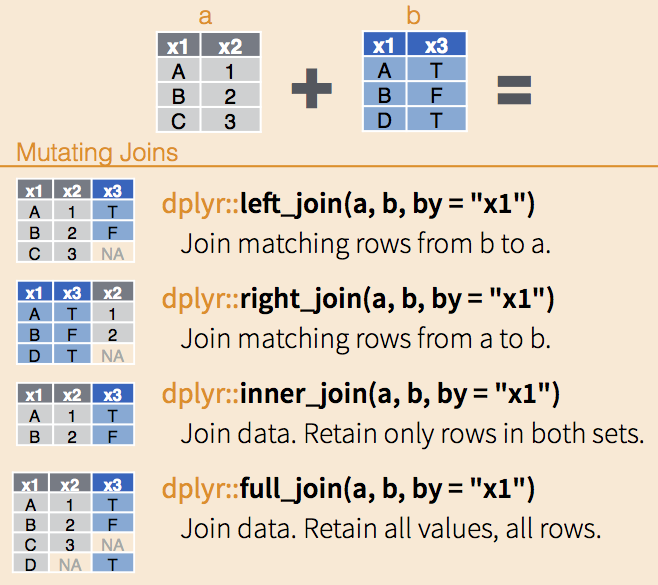
Figure 5.1: Different joint options from dplyr. Adapted from cheatsheet.
class(annotatedPeak) # this tells us the class, which type is it?
annotatedPeak_df=as.data.frame(annotatedPeak) # we will change it to data.frame to have an object we can manipulate better and write to a table
annotatedPeak_df=left_join(annotatedPeak_df,GeneNames, by="feature") #What is this doing?
## [1] "GRanges"
## attr(,"package")
## [1] "GenomicRanges"5.5.5 Explore and export the table
We can now see how the table looks like and export it as a .txt table so we can explore it outside R.
as.data.frame(head(annotatedPeak_df))#how it looks?
write.table(annotatedPeak_df,file = "../macs2_analysis_p0.05/ChipPeakAnno_results.xls",row.names = T,col.names = T,sep="\t") #this is writing the table, look in your directory and try opening it with excel.
## seqnames start end width strand length abs_summit pileup X.log10.pvalue.
## 1 chr2L 34224 34348 125 * 125 34306 20.88 2.75497
## 2 chr2L 34224 34348 125 * 125 34306 20.88 2.75497
## 3 chr2L 34965 35180 216 * 216 35108 23.26 3.33362
## 4 chr2L 34965 35180 216 * 216 35108 23.26 3.33362
## 5 chr2L 40369 40577 209 * 209 40492 30.42 7.01721
## 6 chr2L 40369 40577 209 * 209 40492 30.42 7.01721
## fold_enrichment X.log10.qvalue. name peak
## 1 1.97319 1.12350 PeakAna_clk_Ip_vs_INP_peak_1 00001
## 2 1.97319 1.12350 PeakAna_clk_Ip_vs_INP_peak_1 00001
## 3 2.02190 1.65302 PeakAna_clk_Ip_vs_INP_peak_2 00002
## 4 2.02190 1.65302 PeakAna_clk_Ip_vs_INP_peak_2 00002
## 5 2.83398 5.05903 PeakAna_clk_Ip_vs_INP_peak_3 00003
## 6 2.83398 5.05903 PeakAna_clk_Ip_vs_INP_peak_3 00003
## feature start_position end_position feature_strand insideFeature
## 1 FBgn0031209 21823 25155 - upstream
## 2 FBgn0031209 21823 25155 - upstream
## 3 FBgn0031209 21823 25155 - upstream
## 4 FBgn0031209 21823 25155 - upstream
## 5 FBgn0267987 54817 55767 + upstream
## 6 FBgn0267987 54817 55767 + upstream
## distancetoFeature shortestDistance fromOverlappingOrNearest SYMBOL
## 1 -9069 9069 NearestLocation Ir21a
## 2 -9069 9069 NearestLocation Ir21a
## 3 -9810 9810 NearestLocation Ir21a
## 4 -9810 9810 NearestLocation Ir21a
## 5 -14448 14240 NearestLocation <NA>
## 6 -14448 14240 NearestLocation <NA>5.6 Annotate with ChIPseeker
We are going to use now ChIPseeker, another chip-seq annotation package. We need to do again many things, like extracting the Gene-names. Luckily we already did part of the work.
library(ChIPseeker)

#we will use the Genomic Ranges object created previously and the txdb also
peakAnno <- annotatePeak(peaksGR, TxDb=txdb, verbose=FALSE)
peakAnno_df <- as.data.frame(peakAnno)

GeneNames = AnnotationDbi::select(org.Dm.eg.db, c(as.character(peakAnno_df$geneId)), "SYMBOL", keytype = "ENSEMBL")
GeneNames$geneId=GeneNames$ENSEMBL
head(GeneNames)
## ENSEMBL SYMBOL geneId
## 1 FBgn0031209 Ir21a FBgn0031209
## 2 FBgn0031209 Ir21a FBgn0031209
## 3 FBgn0267987 <NA> FBgn0267987
## 4 FBgn0051973 Cda5 FBgn0051973
## 5 FBgn0051973 Cda5 FBgn0051973
## 6 FBgn0051973 Cda5 FBgn0051973GeneNames=GeneNames[,-1]
peakAnno_df=peakAnno_df %>% left_join(GeneNames, by="geneId") #this is merging the two tables by the column Geneld5.6.1 Explore and Export the output
If we look at the head of the file we can see that we have a different annotation format for the peaks and that we actually have a distance to the TSS.
We will save this file as well.
head(peakAnno_df)
write.table(peakAnno_df,file = "ChIPseekerAnno_results.xls",row.names = T,col.names = T,sep="\t") #try looking at it on excel or any other spreadsheet editor, what are the differences you see with the previous one?
## seqnames start end width strand length abs_summit pileup X.log10.pvalue.
## 1 chr2L 34224 34348 125 * 125 34306 20.88 2.75497
## 2 chr2L 34224 34348 125 * 125 34306 20.88 2.75497
## 3 chr2L 34965 35180 216 * 216 35108 23.26 3.33362
## 4 chr2L 34965 35180 216 * 216 35108 23.26 3.33362
## 5 chr2L 40369 40577 209 * 209 40492 30.42 7.01721
## 6 chr2L 57282 57429 148 * 148 57365 22.07 3.47781
## fold_enrichment X.log10.qvalue. name
## 1 1.97319 1.12350 PeakAna_clk_Ip_vs_INP_peak_1
## 2 1.97319 1.12350 PeakAna_clk_Ip_vs_INP_peak_1
## 3 2.02190 1.65302 PeakAna_clk_Ip_vs_INP_peak_2
## 4 2.02190 1.65302 PeakAna_clk_Ip_vs_INP_peak_2
## 5 2.83398 5.05903 PeakAna_clk_Ip_vs_INP_peak_3
## 6 2.08079 1.77350 PeakAna_clk_Ip_vs_INP_peak_4
## annotation geneChr geneStart geneEnd
## 1 Exon (FBtr0078163/FBgn0051973, exon 7 of 13) 1 21823 25155
## 2 Exon (FBtr0078163/FBgn0051973, exon 7 of 13) 1 21823 25155
## 3 Exon (FBtr0078163/FBgn0051973, exon 5 of 13) 1 21823 25155
## 4 Exon (FBtr0078163/FBgn0051973, exon 5 of 13) 1 21823 25155
## 5 Intron (FBtr0078163/FBgn0051973, intron 2 of 12) 1 54817 55767
## 6 Promoter (1-2kb) 1 25402 59268
## geneLength geneStrand geneId transcriptId distanceToTSS SYMBOL
## 1 3333 2 FBgn0031209 FBtr0113008 -9069 Ir21a
## 2 3333 2 FBgn0031209 FBtr0113008 -9069 Ir21a
## 3 3333 2 FBgn0031209 FBtr0113008 -9810 Ir21a
## 4 3333 2 FBgn0031209 FBtr0113008 -9810 Ir21a
## 5 951 1 FBgn0267987 FBtr0347585 -14240 <NA>
## 6 33867 2 FBgn0051973 FBtr0078163 1839 Cda55.6.2 Positive controls.
We can now explore the data back at IGV and see if the genes we get a significantly enriched for this TF are actually enriched.
Lets think about some controls we can do with the data. Which is the protein we are analyzing? Is there any gene we already know that protein might be regulating?
Well, yes. We are analyzing Clk, that happens to regulate tim.
So, making it more general: Other option to see if our analysis and the data in general make sense is to go to previous literature and see what genes we know that are regulated by this TF. Then, we expect them to be enriched in our analysis.
peakAnno_df_tim=peakAnno_df[which(peakAnno_df$SYMBOL=="tim"),] #What we are doing here?, remember Lab 2!
peakAnno_df_tim=peakAnno_df_tim[order(peakAnno_df_tim$X.log10.pvalue.,decreasing = T),] # we order them by log10(pval), what that really means?

as.data.frame(head(peakAnno_df_tim))
## seqnames start end width strand length abs_summit pileup
## 3983 chr2L 3504149 3508352 4204 * 4204 3507246 140.77
## 3984 chr2L 3504149 3508352 4204 * 4204 3507246 140.77
## 3985 chr2L 3504149 3508352 4204 * 4204 3507246 140.77
## 3986 chr2L 3504149 3508352 4204 * 4204 3507246 140.77
## 3987 chr2L 3504149 3508352 4204 * 4204 3507246 140.77
## 3988 chr2L 3504149 3508352 4204 * 4204 3507246 140.77
## X.log10.pvalue. fold_enrichment X.log10.qvalue.
## 3983 34.61634 3.45781 31.83545
## 3984 34.61634 3.45781 31.83545
## 3985 34.61634 3.45781 31.83545
## 3986 34.61634 3.45781 31.83545
## 3987 34.61634 3.45781 31.83545
## 3988 34.61634 3.45781 31.83545
## name annotation geneChr geneStart geneEnd
## 3983 PeakAna_clk_Ip_vs_INP_peak_539 Promoter (<=1kb) 1 3493986 3507218
## 3984 PeakAna_clk_Ip_vs_INP_peak_539 Promoter (<=1kb) 1 3493986 3507218
## 3985 PeakAna_clk_Ip_vs_INP_peak_539 Promoter (<=1kb) 1 3493986 3507218
## 3986 PeakAna_clk_Ip_vs_INP_peak_539 Promoter (<=1kb) 1 3493986 3507218
## 3987 PeakAna_clk_Ip_vs_INP_peak_539 Promoter (<=1kb) 1 3493986 3507218
## 3988 PeakAna_clk_Ip_vs_INP_peak_539 Promoter (<=1kb) 1 3493986 3507218
## geneLength geneStrand geneId transcriptId distanceToTSS SYMBOL
## 3983 13233 2 FBgn0014396 FBtr0077567 0 tim
## 3984 13233 2 FBgn0014396 FBtr0077567 0 tim
## 3985 13233 2 FBgn0014396 FBtr0077567 0 tim
## 3986 13233 2 FBgn0014396 FBtr0077567 0 tim
## 3987 13233 2 FBgn0014396 FBtr0077567 0 tim
## 3988 13233 2 FBgn0014396 FBtr0077567 0 tim5.6.3 Plots
This package has some useful plot functions so we can explore the results more easily.
First we can see the peaks over the chromosomes. For that we use the function covplot. Its name comes from “coverage plot”.
What do you think about the results? Do they make sense?
covplot(peaksGR, weightCol="X.log10.pvalue.",chrs=c("chr2L","chr2R","chr3L","chr3R","chr4","chrX","chrY"))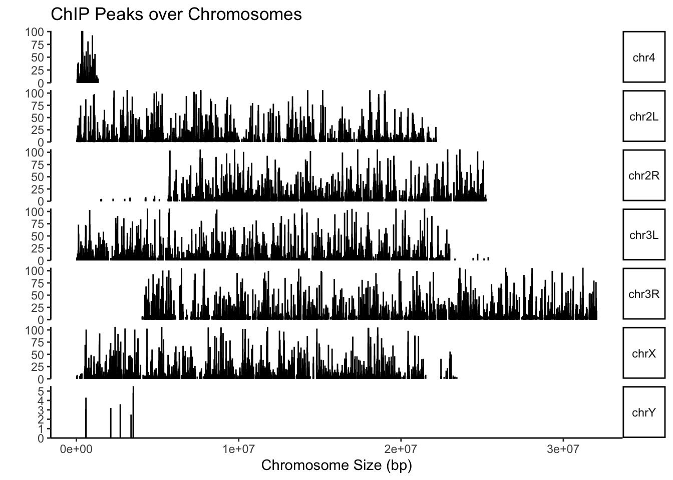
Figure 5.2: Coverage plot.
And then a general distribution of the peaks in relation with he transcription start site (TSS). For that we use the function peakHeatmap and plotAvgProf2.
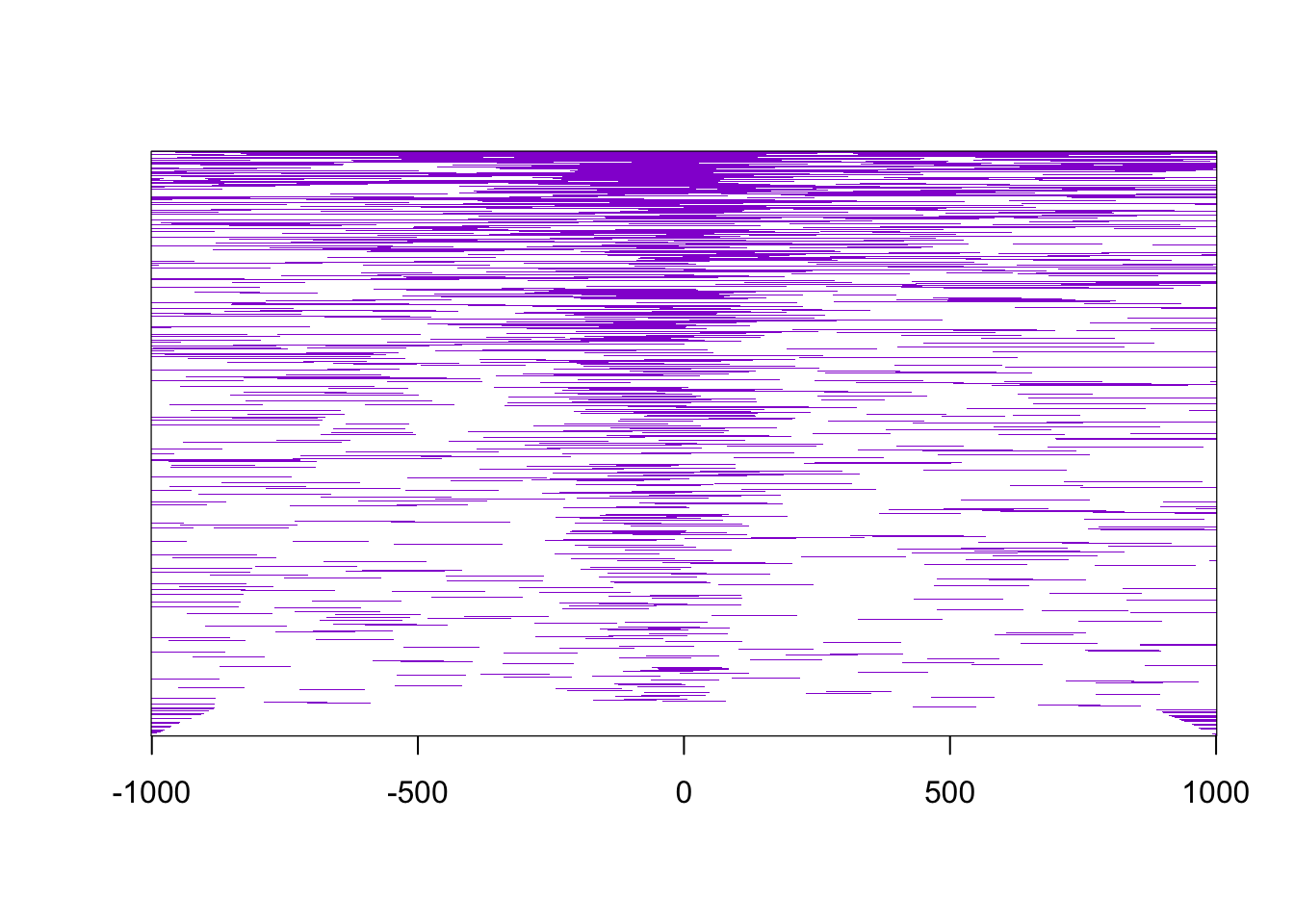
Figure 5.3: Peak heatmap.
## >> preparing promoter regions...	 2020-08-30 21:12:31
## >> preparing tag matrix...		 2020-08-30 21:12:32
## >> generating figure...		 2020-08-30 21:12:37
## >> done... 2020-08-30 21:12:41plotAvgProf2(peaksGR, TxDb=txdb, upstream=1000, downstream=1000, xlab="Genomic Region (5'->3')", ylab = "Read Count Frequency") #Try exploring the options of this function. 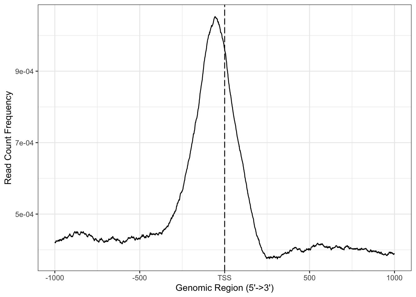
Figure 5.4: Average coverage plot.
## >> preparing promoter regions...	 2020-08-30 21:12:42
## >> preparing tag matrix...		 2020-08-30 21:12:42
## >> plotting figure...			 2020-08-30 21:12:45
5.7 Sequence Motif analysis
Another goal now is to analyze this peaks and see a pattern enrichment and see if we can find a Binding Motif for Clk in fly head.
This is basically DNA analysis, so we will have to figure out the regular DNA motifs and see if there is any specific enrichment.
For this we will use the following libraries:
5.7.1 Put the peak sequences in fasta format
To parse the corresponding sequences from the reference genome, the getSeq function from the Biostrings package can be used. The following example parses the sequences for each peak set and saves the results to separate FASTA files, one for each peak set. In addition, the sequences in the FASTA files are ranked (sorted) by increasing p-values as expected by some motif discovery tools, such as BCRANK.
library("Rsamtools") #we will use the Rsamtools package for this.

peaksGR <- peaksGR[order(peaksGR$X.log10.pvalue., decreasing=TRUE)] #order the peaks according to pvalue.

as.data.frame(head(peaksGR))
## seqnames start end width strand length abs_summit pileup
## 1 chr2L 3133811 3135424 1614 * 1614 3134481 140.17
## 2 chr2L 3136702 3137388 687 * 687 3136981 140.77
## 3 chr2L 7649255 7651111 1857 * 1857 7649737 140.77
## 4 chr2L 7661000 7661782 783 * 783 7661451 140.77
## 5 chr2L 14249821 14250599 779 * 779 14250165 140.77
## 6 chr2L 18077759 18081655 3897 * 3897 18078127 140.77
## X.log10.pvalue. fold_enrichment X.log10.qvalue.
## 1 106.096 12.73315 97.93874
## 2 106.096 12.78695 97.93874
## 3 106.096 12.78695 97.93874
## 4 106.096 12.78695 97.93874
## 5 106.096 12.78695 97.93874
## 6 106.096 12.78695 97.93874
## name
## 1 PeakAna_clk_Ip_vs_INP_peak_474
## 2 PeakAna_clk_Ip_vs_INP_peak_477
## 3 PeakAna_clk_Ip_vs_INP_peak_1071
## 4 PeakAna_clk_Ip_vs_INP_peak_1079
## 5 PeakAna_clk_Ip_vs_INP_peak_1893
## 6 PeakAna_clk_Ip_vs_INP_peak_2290pseq <- getSeq(FaFile(file = "../macs2_analysis_p0.05/dm6.fa"), peaksGR) #extract the sequence of the peaks using the genome fasta file dm6.fa and the genome-ranges in the object peaksGRWe can now see how the pseq object looks like.
## x
## 1 ACCCATTAAATTGTCAATATTACTTAAGCCCTTTATGGTATTGGAAACTCCCGTTTCACATAATTAAACATGGAATGCAGCAAAAAATTTTCCGTGCAATTGCAAATGGCATTTTACGAGAGAAAATTGTTGACAATAATGAAGCTGATGAACATTTGTGGTTGTGTTCATTGTCATTGTTGCTGCGTTAGTTATTCTACCATCGGTTGGGGTGCATTTGGGCCAGTCTGGAACTGTTTGCGTCATTGTTCAGTTTTAGTTCTCTGCGGTTGCCTGAAATTGTCGTAATGCATTTACGGACATCGCACACACATGTGGCCCAAGTGCGGTTTTGTAGCTGGAAATGTTGGCTGTGTACTGTAAACAAGATTTTAGCAAACCCACTTGCATTTCTCCTGGGGGTCATGTGTCAGCACTTATAATTTTGTTTAAAGAACTAAGAGAAAAATGTCCACTATCTAGAAAATCATTACTATCAAAAAACCCAATTTATATCAGTAACGTTCGATTTCTAAACTCATATTGACATTTTTGTATGTATATTATGTATGTATATAAATGTTCATATTTGTTTCCCTTTTGGTTGCGTACCTAACCACCACCTATAAATTAGCCCGTTCTGCCAATATTAGCCCTTTCATATCTCGTTACTCATACGCCACGTGGTCACGTTTTTGCCTAAGCTCTACGTAGCTGCACTCGCTGCACTTTCCGCTTACGTTTTGTTATTATTTTCCCCAGTACTCGTTAGCCTTGTCTAGTGCCAAAATGAAATGACAATGTTTTCCCAGCGCACAGAACTCAAATCGTAAATCATTTTCTTTTTTTTGGGGTGTTGGCAAAGGTAAACAATGTCACATAGGAGCCCGCAGTTGTCTGTCAGTAGAGAAAAAGGCAAAAAGATTAGAGATATATGGACTGCGGAGAGCGGGGCAGAATGCGAGATATATAGCAACTCAAGTTTGTGTTGCCACGAACTTTGACAGTTACATGCGCTGCACCATTGCAGAATGACAAACGAAGGCGAAAAAAGCCATGAGTTGCACAAAATGTATTTATCTGTCATTCCAGTTTTCACTTTCGCAAAAAGTGGTAGATTTTGGGTTTTGTGTGGAATCATATCTAGCTTTATAGCTCTTGGGGAACTATAATATGACTTAAATACCAAATATTTATATACTCAAGTTTAATATAATACATTTCACGTAGTTTTAACGCAAAACGGAATATGCTAGAATTTATCTTTTCCACTTCGTTTCCCCTCTGATTCTCGCACTTTCCCCCAAACTCTCGGCGTTTGTGTGTGTGCCTGTCTGGCTTTTCTTTTTCGTCTCCGTTCGTGACAGCTTGTTTTTTTGGGGGCGTGGCGAGGGGCGGAAGGGGTTGGGCATTTGGGTCAACTATCGACTGCAATTTGAGCCTTTCAAACTGTCGCCGACACAAAACGAAGGGCTCAGCTGAAAAAAAAAACACACAGTCAGGCAGAGTAAAAGTTGCGGAAAGTGTGACAGCAACTCATTGCAGATGGACATTTGCCGAGTCTGCTGGGAATCCCCTCAAGTGCTCTGGAAATTTGATTTCGATTTCCATATGATTTTGATTTGGCCAGCGAAC
## 2 CTTCCCCTTTTATTACTGTTCCAAGGACATTCAAATTAAGCATTCATTTGCGGTGATATCACCGGCTTTAATGCTCTGAACTCCACGAAGAGTTGACTAACCTCGAACTGTGCTACATTTTTTTATGCACCTCCATCATACACACATTTTGTCGTGTAATTTGCACGCTGAGTCTATTAAATGCACTGCAACCGAGTTGTGTCAGCACCTCAGGTGTACAGAGCTTTCACTCACACTCATATACGATTCATAAACATTTGTTGTGGCGCCCAACGTGGGGCATGAAATGCGACGTGTTACACAAGTGGGAAGAAGAAGGTGCAAGTCATTAAGTAAGCTTGTTTTTGTTCTGATTTTTCTCGTTGTTTTCAGGGAAGAGGCCATAAAAGCTTCGTGCGCCACGCACACATGCACACATAATTATAATGGGCATTAAAACGGACGCCTGTGGCCTAACTCTTAGTTTGTCTTGTTCGCCAGCAGGCTTCTTAACCCTCACACTGTCCAACTTGGCTACCTCTGAGTGCTTTATGGCGCAACTGGTAGAATGATTCGCCGAGCATAATATTTAACTCGGAATTCCCTGCTAAACGCACATAATGTCTGCCCAAGACAGTCCCGGTTCCCAGCGGCGAAATTCATTTTCTTGTCGCTTACAAATTATTTTAAAGGTATTTAAAGTTAGAT
## 3 AAAACAGAAGCTCTAGCATTGTTGTGATACATTAAAGAACTTTACTGACCTGGCCAATTTGTGGATAGTGCTGCAGCTCCATCTCGAGCACCCGCATGGACGGCTTGGGGGTTGTCAGCTCCTGGCCCGTGCACATCTCGTAGAGCAGGTGGCCAAAGCAGACGATGTCCACGTTCTCGATCTCGGTGACCGAGCGGGACCACATGACGGCGTTAATGCGCGAACTGAGGCCCAGGAGGCCGTTCTCCAGGCCCGATAACCTGATGGGTGAAAAACGGAATAAATGTTACGGAAAATGCATAATTAAATGGCGGACCCCTTGTGCTTTCCTTCCCTTTTGTTTCGGTCTTAATTATGCAACATATTCGATGGCTACCCTGCCGTATATTGATGGCCAACACGTGGAAACGTCGGCCGCAAAGTGTCTACTTTTATGGATTTATGTGCGAGCGAGAGGGAGCAGGTATCATCTGCTATCTCTTTCCTCACTGGCCATGTGCCTTAATGACAAAGAGCGTATGTCAGACCTGATATGACAATATTATGACACTCTACACAACACAGCGCTGTATATTGCGGATTGGTTGGGGCTTTTGGTTCGAGGGTCCTGCCGGCATTTCCTAGTATTCATTAGGCCAAATGTGGCTGACTAGTTGGAAAGGTATTCCGAATTGGCTGACAATAGAGGTTCTGAAGATGCTAGTTGTCGTGTGCTATAGTTTATTGGCTTTTGTTGCCAGTTGCCTTTGTTTATTTTATGATCATTTTAATTAGTTTTGAAAATCAGATAAGTATAAATATACGAAAAAAAATCATTTGGGCTTAAAAAAGTTCAATACAAATTGTTGAGTCAACAGGTTACTCCAGAAGTATTTGTTGTCAAATTTACTATCAAATATAAGCATGTTTTTCTTTAGCTGTTATAAAACAATAAAAGCGTTGTGCAGACATTAAATGCTTTCTTTTATTGTCATTGCAAATATCCTGAAATTCTTCACTCAATTTCACTTGAGCAAGCATTTTCTTTTCTACTTCGTCAATCAGCTTTTCAGCTTACTAAATTCCATTTTACCCGTTTTCTTCACGTTGGTCTTTCAACTTTCCTGTGGCCCTATCAATAGCTGTACGTATGTATAAGCAATTTATATGAAAATCAGCTTTTCAATGCGCACAGCGATACCCTGGCGACGAAGGCAGCAAAATTGGGTCATGCACTTGGCGCAAACTTGAACGCAGAAAATCCGCACTTTAATCGACTTTCACCTATAGGAATTCTAGCTTGCAGATCCCACCCTCTTTTAGTCCCGTCCCTGGGCTGCAATATAACCATCTTTTTCGCCGACCATTTATTTTTAAAATGGCAAAAAGCTTAAGCTTTATTTTTGTTACACCCATTCGATGTTTGCAAGTGGGTGGTTTAGTGGGTGGCGCTTACGCGTTGTCGCACAGCAGCTACATGGATAGGAGGGGGCCAGTCAGGGGCTCACGAAACAGGGACATGCATTTAAAGTGCCCTGAAATGGGCAACGATTCTGGGGAATTGCTTTTAATTTGCCATTTAGGCTGAAATCGATGTCGGTTCTATTTGGGTGAATTTTGAATGACTGAAATTTTGCAGTGGAGATAGGGGGGCAGGCCACCGATTCGATATAAAATATTGCAGCCATTATTAAATTAGTTAACAGTTGAGTGGGTCCCAATCGACAACGGACTCACCTGGCTGCCCCGTTCTGCAGGATGACATTGCCGCTGTGCAGGTGACCGTGAAGCGGAAAACCGCGCTCCTTCAGGAAGAGCAGTGCCTCCAGAATCTGTCGTCCCAGGCGCTGCACCTGGCTCACCGGTAAGCCATTTGGC
## 4 GGCGCCAACAATCGTAATGGATCCTGGCATGAAAACGGGATGAGGAGACCCAATGGTCACCGCCCTCTAAATGCCGAAAGTCAACTGCGTCATTGTTTGGGGAGAACAGGCCAGCTCCAGCTGAATTTCCTCGATTTTCCGAGGGGTGAGATAAAGGGCCCCGGGCCAGGATGGCCAGGCCCATTTCCAGTGACCTTGCATCATTAACTTAATTGCTCAAACAGTAGTCGGTCCGTCCAATTGCCGGGCTGAATTATTCAGTTGTTCTGCTCGGCCAACTGGCAATTTTGCGTCTTTACTAATGTCACCACAAGCTCATAGAGGAAGCGCTGTCTCTCTCTATTCGGCGCTGCACTGGAAAAGCCATCCGACAGAACCGTTTTTCCATGGGGGCCGGTGAAAATCCCCCACGTGCATTCGGTGTGGTCGTTGGCCCGTTCACGTTGTCCCCCCATTTTAAAGGGGCGTCACGTGTAGCGGGGCTTAGTCCCCCCCACCACAATTTGACATTTTTTACGAAAACAAAATGCAGAGATACGAAGAGAAAAACCAGGCCCAAACAATTTTCACCGGACTAATTGGATTCAAGAGTTTTCCTGCTGCGCTTTTGTCAACGCATATTGCAACAGAAATATTCATATTTATTTATATATAAAAATTCACTGTCAGTACAGCCTAGCCTATAGTTGAATACATACCTGCATCGTCTTATCCAGTATGAAATTACAACAATTCCACCCAATATCAAACCACCTAAGGCACACCAAAAGAGGGTCTGAAAAG
## 5 AGGAAAACTCCTAACAAGCTTTAAAAACCTAGCAAGCTAACTACCTTTTTCTTAATTCTCTGGTTCGTTTCGCACACCTGATTAATGGGTTAATGTATCTATTTTTATGCACCCAGCTGCCACTCAGTTGGCTTTGACTGGTCTCGGGGATAAGTGGCAAAGAGGCCGGCTAATCAGGCCCAAAGGTAAAGCCAAAGCCAAAGCCATGAACCAACGAACCGCCCAACAGCCCAACCACCGAAACGCCCCACCCATCCGCTGGTGACCCACTTGAGCATGCACCGCTCGTGACATTGGGCAGGGAAACGTGCAGAAGCGACGGGAAATCGACAAGAAGACAAACAAAACAGCAAAACGTGCAGAACGTCACTTTCGGGCCGCCTTTTTGTTGTTAATTTAGAGAGATGCGTCACAGCGAAAAGTGTTAAGAAAGAAATGCGCGGAAAATCAGGAAATGTAAGCGGTGAGAACTGCGCATTAAGCATCGCATTGCATCGCACGGCAAAACGCAGCCAAATAAAGCGAAACAACAGCGGAGACAGGCGCAATGTTGACAATTGTTGAAACTGACAGTTTGACGTTTTAACTCACGCGCCAAACGCCAAACGTCAAACGGCAGCAACAACCAACACAATATCAACATCAGCAACATAGTAATACGTTGTACGGCCAAACGGCAATCTAGGCAAATCCACCGAGTAGACAACTCAATGAGCCATTTTGATGGACACCTCCGACGACAGCTGTACGGCACACGAATGTATATAATGCATATTCAT
## 6 TGGAATACTTGGAATTTATTAAGTACCTCGTTGTTATAACTAGTAGTTGTCTCCAGTTAACATAAAGCTATTATAAATGTCATAATAAACAACCGCTTATCAGTACTTAGCCGACGAGTGCTTAGGGCTCAATTAAATTAACAACAATTACGTAAATGGAAAAGAACAAAACCCACCACGTAATGTTTGGGTTTAAATACGTCATCCTAGGCGGAAAACAACAAACCAAAATACGCATACTAAATCGATTTCTCGAGCTATTTCTGTACATTCACCTGTCCTGCATTGCTAATACGCCGTGTTGCTCGCGCGTTATTTAATGTTTGAGCCATCGATGTCGATGTCGTGCTGCAATGTCAATATCAAAGACACTGCGCACAGCAAGGTTGCCGAAGCCGTAGTAGTTTACCGCCGTGCAATTGCTGAATTTCTGCTGTGCGGCTAATTGAATTTAGAGGGGCGACAGGTGCCACAATGCCAGGTATAAATGCCGGATTGCCAAAGAGCGCTAATTAATAGCCTAGTGGACCACGCAACGCGGCGTATACCATCGAGAACGAGCGCGAAACGTTAAAGGCACATCCAAAGTTTAAACTATTTCCGCAGAGATTTTGATAAACAGCTCCAAAATGGTGGTCAATTTCAAGGTGTTCAAGAAGTGTTCCCCGAACAACATGATCACGCTCTACATGAACAGGCGTGATTTTGTAGATTCCGTGACTCAGGTGGAACCCATTGGTAGGTGTCACAGACCGAAACCCTTGAGCAATGGGATTTACGAATGAGGAAATCCATCAAAAAATAAATTCGTGTAGGAATTGGTACCCATATTCGATTGAAGTATCTTATAGTTTGAAAATAACTTCAGTGTAACTTTTGTTTCAACTTAACACATTGGAATTTTTAATACCTTCCTTGAAAAGTGATATCAAATCAAAATTATATTATAAAAACTCCATTTCGAATCTGCATATGCCGACCAGCAAATATAAACTCAGGGAGTTATTCAAAATTGCATCTGAATTCAATAGCCCAGGGAGTTAAGTTAAATTGGCTGCGCTAGCAGCTAACCAAGTTCATCGATTACGCGAGCAAGCAAACCAAGAGGCTGGGCGCTTGTAAATAATATTCTCCAATTAATAAGCGTCCTCTTGCAGATGGAATCATTGTGCTGGACGATGAGTACGTGCGCCAGAACCGCAAGATCTTCGTGCAGTTGGTCTGCAATTTCCGATATGGGCGCGAGGACGACGAGATGATCGGTCTGCGGTTCCAGAAGGAACTGACCCTGGTCTCGCAGCAGGTGTGCCCACCCCAGAAGCAGGACATCCAGTTGACCAAGATGCAGGAGCGTCTGCTGAAGAAGCTTGGCTCCAATGCCTATCCCTTCGTGATGCAGATGCCACCAAGCTCGCCGGCCTCGGTGGTTCTCCAGCAGAAGGCCAGTGACGAGAGCCAGCCCTGCGGAGTCCAGTACTTCGTAAAGATCTTTACCGGAGACAGCGACTGCGATCGATCGCATCGCAGGAGCACCATTAACCTGGGCATCCGCAAGGTGCAGTACGCACCGACCAAGCAGGGCATCCAGCCCTGCACCGTCGTTCGCAAGGACTTCCTTCTGTCGCCCGGAGAGCTCGAACTGGAGGTCACCCTCGACAAGCAGCTGTACCATCACGGCGAGAAGATCTCGGTGAACATCTGCGTGCGCAACAACTCCAACAAGGTGGTGAAGAAGATCAAGGCCATGGTGCAGCAGGGCGTCGATGTGGTCCTGTTCCAGAACGGTCAGTTCCGCAACACGATCGCCTTCATGGAGACGAGCGAGGGATGTCCCCTGAACCCGGGATCCAGCCTGCAGAAGGTCATGTATCTGGTGCCCACCCTGGTGGCCAATTGCGACCGCGCAGGCATCGCCGTTGAGGGTGATATCAAGCGCAAAGACACAGCTCTGGCCTCGACCACACTGTGAGTAAAATTTATTCACATCATAGCTTAGCAGATGAAACATTAATATTATACTCTATTAAGTATCAACTTAAAATCATACCATAAAATCAATCAAATTTTAAAGTTAGGAACCTTTTTAAAAATCGTATTTTCCCGGTGACTAACAGTTCTTTAGCTAAATGTGTTTACAAAATGGCATAAAACGCATACTAATACTAAGTGAAAAATGCATATTTAAAATTCTATTTCAGTATTGCCAGTCAGGATGCGAGGGATGCCTTTGGCATAATTGTTTCATATGCTGTGAAGGTCAAGCTTTTCTTGGGAGCCCTGGGCGGCGAGCTCTGCGCTGAGCTACCATTTATTCTGATGCACCCGAAGGTAATAAAAGGTGTGCCCAAATATTTGAATAGTTATTGAAAGGCAATCAATTATTTACAGCCAAGTCGCAAGGCCCAACTGGAAGCCGAGGGCTCCATTGAGGCCTAAACTGAAAGGGCTACCTCAACCAACGAAAAAAATGGCGTATTTCTACAAGTCAAACCGATTTTTGTAGATCCTAAAAAATGCTGATGTTGCTGAAATGTTCTGAACTGCAGTCGTCGTACTTTTCCTATATAGCAAATCCAATATCCATATATTGTATGTGTGTATGTGTATTATATTTATAACTCAACTAACAATTAAATATGAACAGAGTTTATGTATGTATTTTGGAGTATTCTATTGAATTTAGCACGGTGTATTTGAAAAGGCTCCAGCATTGAAAGTTTGTATGGAATGCGCACTAAATATTTAATAATGTGCTTACGAAGGCATTTCGTAGTATTTGATATCTTGCAATGTCTGCTGATTATGTACATTGAAGTGCAATGGGGAAATCAACAGAAGCCAGTGCAATCTATTCAATTACTAATAGTGGGTCTTGCATTTGTGGCTTAGTAATTCCAATTATTGCTACTCTGAAAAGCCGAGGAGCAGCCTAATTAATACTTGGCCACTATGCTGGAGGAAGTTTACTGAACTGAATTCGAGTAAGGAAAATGGACAATAATTGATATAATATGGTGAGCTTCTTGCTGGACTTTGAAATCGTAAAATTTAAGCGAACACACTTCAAACGCATCCATTTAATTTGTGAATGTTTGCAGTCCCACTTTTAATAAGCACCCAATATTAACGATAACGCCACTCTAATCAAAATTTTCCAATAGTCAGGGTTGAAATACTGATCAATCACGCTGCCAACATTTCGGCAGACCAGGTGGGTAATGAGTTTAAAATGGTTTTGCGTAATGGGATTAATCGAATTTCATTAAGGAAGATTAGATTGCCGTCTTTGGAAGTGATCTTTTATAGTGGCTGACCATAAAAATTGCATTGCAAATACTAATTTAAGCATACATGCTATATAACCGATAAGATGGGCGAGCGTCAAGGCAAAAATAGTTGACCGTATTAATAGTTTAATCAACTAGCTTCAAGTTAATTTATAATGCGAATTAGGAAGCACTCTGGCATGCTATTAAAAACTTAAGAACTGATAAACGAAACTTAATTCCTAAAATAAAAATGTACCTAATTACTTTTATATACTATTATAAATAAAATTGTACCATGTATCGTTAAATTTGATTTAGTTACCAAGTGGTATTTGGTACGTGGCAGCATGAAATAGCTACTACTGCTAGTCTGGCTGATTAGCCAGCACTCTCAATAAACTAAGTGCAGCGTTTTGCATTTATCAGGATTTTTGGTACTCTAAACACACACTTAGATCCCAATCACCCCACAGAATAAGTTGAGCAAACCAAACCGAGCTGATTACCACAGTAGACATGATGATTAGCCGCTGCTTTATTTACTAGTGGATAATCTACTAAGCGACGCATGAATAAAAACTCGAGCGATATTTTTCCACTTTGCAGTCGCTCGAAAGCCTTTGTTTCG5.7.2 Find the MOTIFS
The Bioconductor package BCRANK is one of the many available for de novo discovery of DNA binding motifs in peak regions of ChIP-Seq.
The main function we are using here is bcrank. when looking at the documentation we see that:
“BCRANK uses a heuristic search strategy. First a score is computed for an initial short consensus sequence, typically selected at random. The score considers both the number of consensus occurrences and the rank of the genomic regions. Then all consensus sequences in a neighborhood of the start guess are evaluated and the one with highest score is kept as the starting point for the next iteration. When a local optimum is found, the algorithm is terminated and the locally optimal consensus is reported as a result. In order to increase the chance of detecting the globally optimal solution, the algorithm may be restarted several times using different random starting points. Alternatively, BCRANK can be used for assigning scores to previously established consensus sequences. The sections below describe in more detail how the neighborhood, scoring function and start guess are implemented.”
We will use 25 restarts and a penalty for both repetitive sequences and non-canonical letters.
P1 - Penalty on non-specific bases. Let l be the length of the consensus sequence and b the total number of fixed bases (A, C, G, T) in the sequence. If there are no fixed bases, b is set to 0.5. The penalty is then defined as P1 = b/l. P2 - Penalty on repetitive motifs. Let rn, n ∈ 1, 2 be the number of input DNA regions that contain at least n occurrences of the consensus. Then P2 = 1 − (r2/r1).
set.seed(0)
BCRANKout <- bcrank("peaksGR.fasta", restarts=25, use.P1=TRUE, use.P2=TRUE)
5.7.3 Explore the results
Then we can also see the results, we will se the results that are in the top.
We can first explore the results: the matrix shows the proportion of each letter in each possition for thar specific motif.
##   Consensus    Score
## 1     CACGT 663.2068
## 2     CACGT 648.6057
## 3    GCACGT 550.5658
## 4    ACGTGC 536.9913
## 5    CAAAAG 491.8869
## 6    AAAGCG 491.6031
##
## An object of class "BCRANKsearch"
##
## Search path, starting from SHVWHRYYDT:
##
##     Consensus     Score
## 1  SHVWHRYYDT  26.19329
## 2  SHCWHRYYDT  99.05250
## 3  SHCWHRTYDT 147.47039
## 4  SHCWHRTTDT 178.46498
## 5   HCWHRTTDT 203.84605
## 6   HCAHRTTDT 263.87039
## 7    CAHRTTDT 315.05930
## 8    CAHGTTDT 344.41459
## 9     CAHGTTD 396.57309
## 10    CACGTTD 498.50181
## 11     CACGTT 599.45575
## 12      CACGT 663.20680
##
## Position weight matrix for search result (CACGT):
##
##   1 2 3 4 5
## A 0 1 0 0 0
## C 1 0 1 0 0
## G 0 0 0 1 0
## T 0 0 0 0 1
##
##
## Use methods searchPath(object) and pwm(object) to access object slots.
5.7.4 Plot the results
We can play around with the matrixes and plot them in the known DNA-Logo standard. To do this we will first store the most top motif from toptable. Then we will use the pwa function from BCRANK and the seqLogo function from seqLogo package.
topMotif <- toptable(BCRANKout, i=1)
weightMatrix <- pwm(topMotif, normalize = FALSE)
weightMatrixNormalized <- pwm(topMotif, normalize = TRUE)
seqLogo(weightMatrixNormalized,ic.scale = T)
Figure 5.5: Most significant sequence logo.
We can now do the same with a different function just to show you that you can do the same things with different approaches. This is using function form the seqLogo package.
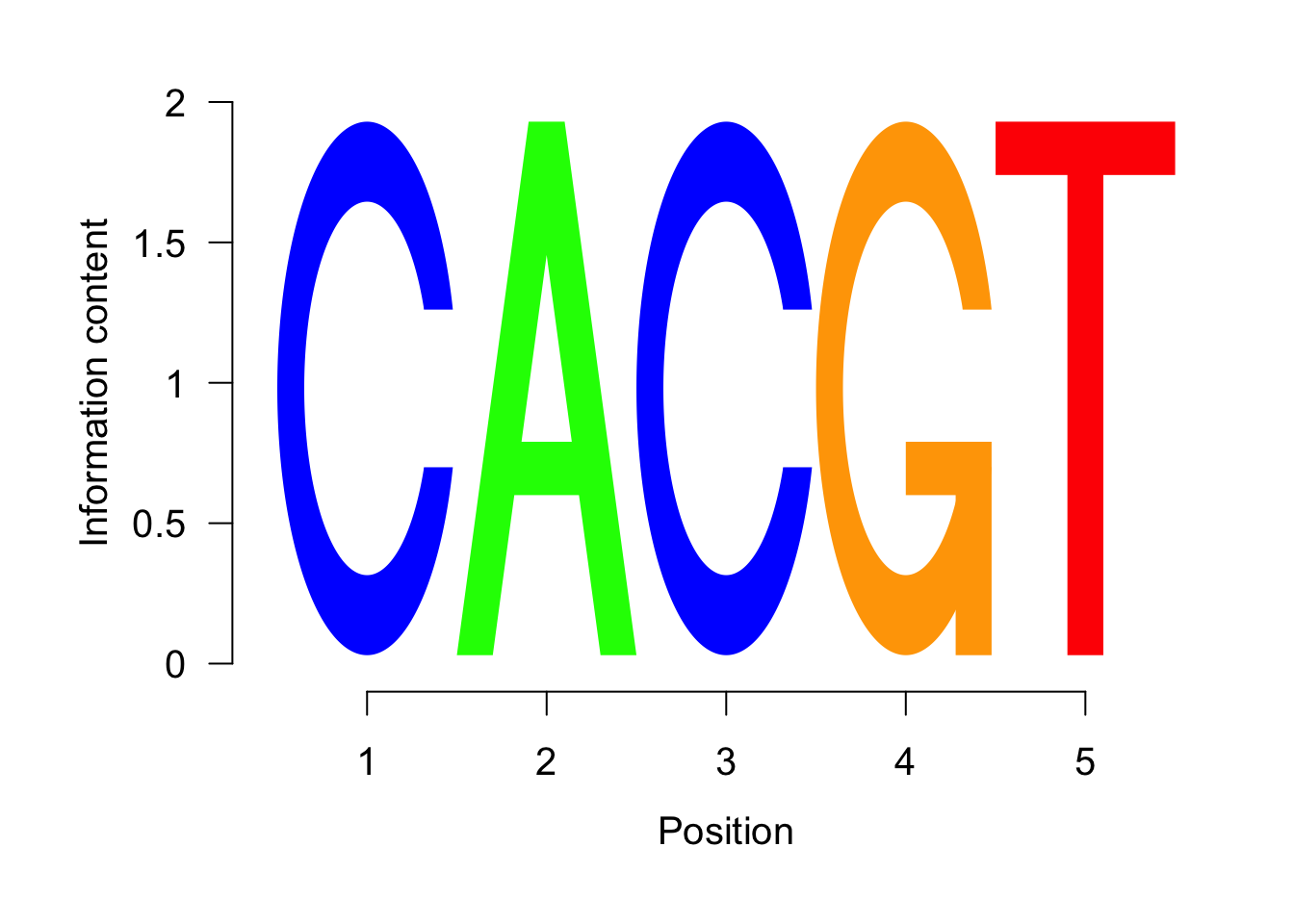
Figure 5.6: Most significant sequence logo.
## [1] "CACGT"We will create a table to be able to analyze the data
##   Consensus    Score
## 1     CACGT 663.2068
## 2     CACGT 648.6057
## 3    GCACGT 550.5658
## 4    ACGTGC 536.9913
## 5    CAAAAG 491.8869
## 6    AAAGCG 491.6031
5.7.5 Plotting with Ggplot2
Now with ggplot we will use a package called ggseqlogo. This will be nice to learn how to install packages from github (you have to use the package devtools and then the function install_github). http://www.bioconductor.org/packages//2.11/bioc/vignettes/seqLogo/inst/doc/seqLogo.pdf
library(ggplot2)
#install.packages("devtools")
library("devtools") #this library is literally called "developers tools" and allow us to do more complex things as downloading packages from github
## Loading required package: usethis5.7.5.1 Create the matrixes for ggplot2
We will first store all the matrixes in a list so we can then just plot them all together and not only one by one.
# Some example DNA sequences, lets try to go together over what is this loop doing
seqs_list=list() #first we create an empty list that we will fill up over the loop
for(e in 1:16){ #we will loop 16 times
  #print(e) #we will print every loop
  topMotif <- toptable(BCRANKout, i=e) #we get the motif number e (ie, the iteration will let us go from top motif 1 to 16)
weightMatrixNormalized <- pwm(topMotif, normalize = TRUE) #do some process with the motif
seqs_list[[e]]<-weightMatrixNormalized #add the processed motif to the list in position e (ie. the loop allows us to fill up the list)
}
5.7.5.2 Plot
We can now, either plot one by one for each position in the list.
# Get first set of sequences
seqs_dna = seqs_list[[1]]

# Plot a sequence logo with the 2 different methods available
p1 = ggseqlogo( seqs_dna, method = 'prob' )
p2 = ggseqlogo( seqs_dna, method = 'bits' ) +labs(y="Information Content") #this changed the name of the `y` axes
grid.arrange(p1, p2)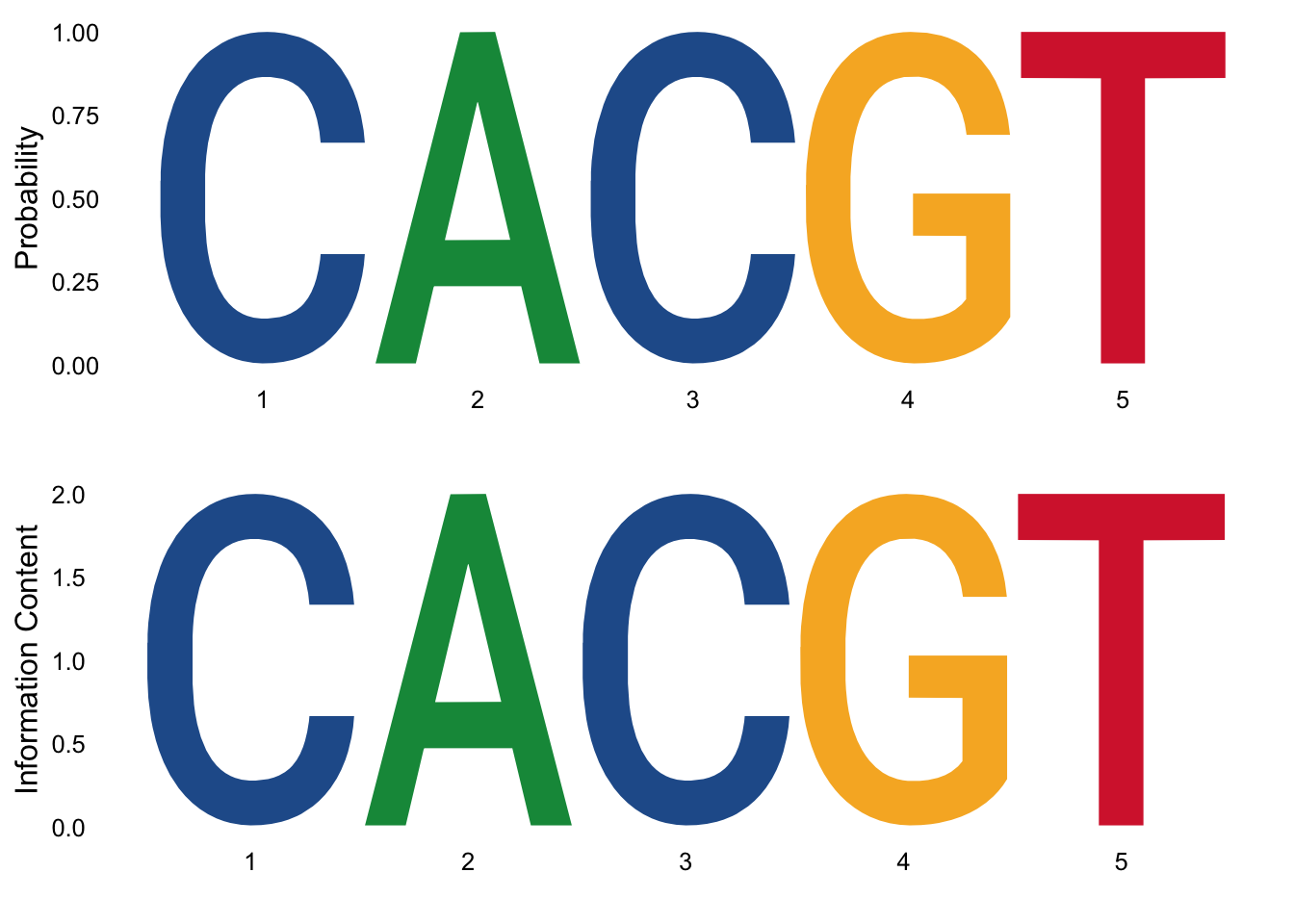
Figure 3.10: Most significant sequence logo in probability and percentage of information.
Or we can plot all together using the facet function to actually separate them.
#Plot all the first 12 sequences
ggplot() + geom_logo(seqs_list,method = 'prob') + theme_logo() +
  facet_wrap(~seq_group, ncol=4)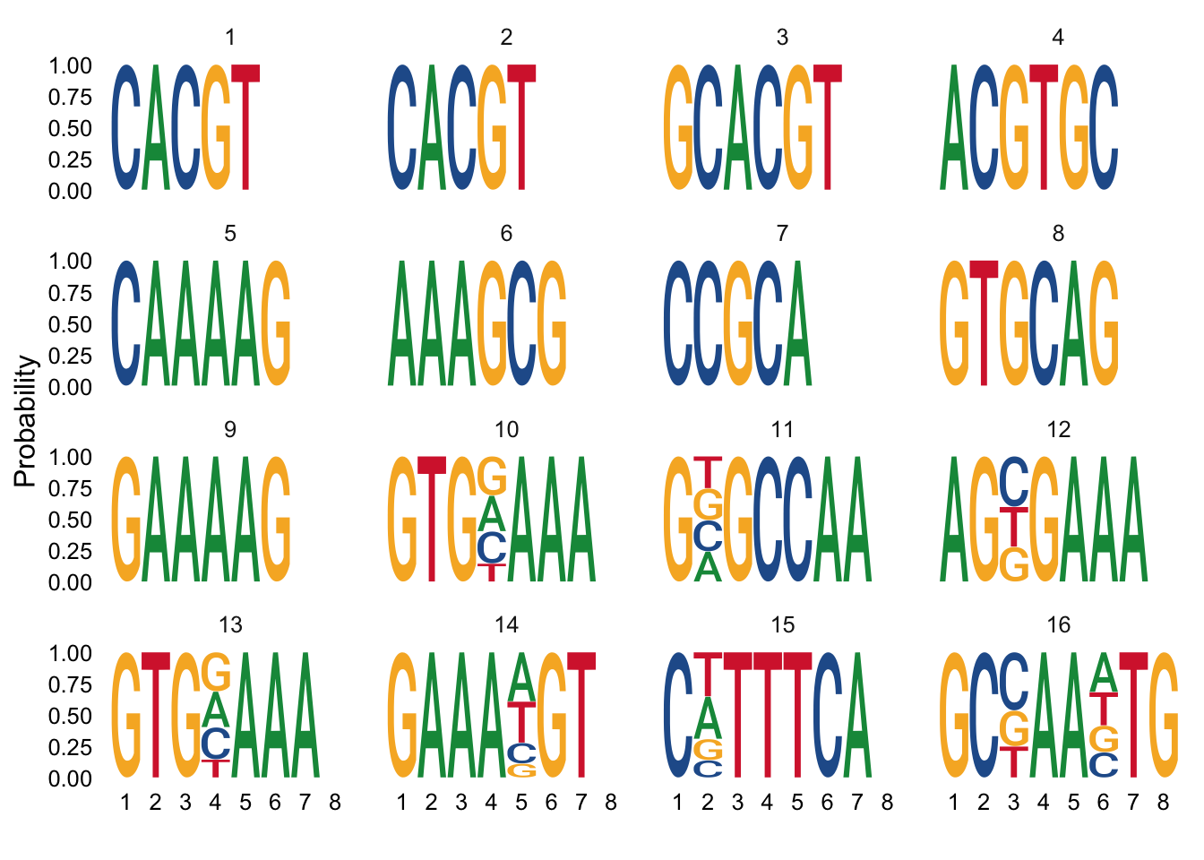
Figure 3.11: Many significant sequence logo in probability and percentage of information.
5.8 Extra: How to solve some common annotation issues.
Lets see some regular problem and how to solve it.
I will show you first a regular problem we can have: annotation files do not correlate with the one previously used for annotation.
txdb <- makeTxDbFromGFF(file="../macs2_analysis_p0.05/Drosophila_melanogaster.BDGP6.92.gtf", format = "gtf", dataSource="dm6", organism="Drosophila melanogaster")
saveDb(txdb, file="./dm6.sqlite")
txdb <- loadDb("./dm6.sqlite")
class(txdb)
## TxDb object:
## # Db type: TxDb
## # Supporting package: GenomicFeatures
## # Data source: dm6
## # Organism: Drosophila melanogaster
## # Taxonomy ID: 7227
## # miRBase build ID: NA
## # Genome: NA
## # transcript_nrow: 34767
## # exon_nrow: 87482
## # cds_nrow: 62757
## # Db created by: GenomicFeatures package from Bioconductor
## # Creation time: 2020-08-30 21:13:02 -0400 (Sun, 30 Aug 2020)
## # GenomicFeatures version at creation time: 1.38.2
## # RSQLite version at creation time: 2.2.0
## # DBSCHEMAVERSION: 1.2
## [1] "TxDb"
## attr(,"package")
## [1] "GenomicFeatures"Now we can actually extract the gene location from the annotation that we created
ge <- genes(txdb, columns=c("tx_name", "gene_id", "tx_type")) #get the genes genomic ranges
as.data.frame(head(ge))
## seqnames start end width strand tx_name gene_id
## FBgn0000003 3R 6822498 6822796 299 + FBtr0081624 FBgn0000003
## FBgn0000008 2R 22136968 22172834 35867 + FBtr0071.... FBgn0000008
## FBgn0000014 3R 16807214 16830049 22836 - FBtr0306.... FBgn0000014
## FBgn0000015 3R 16927212 16972236 45025 - FBtr0415.... FBgn0000015
## FBgn0000017 3L 16615866 16647882 32017 - FBtr0112.... FBgn0000017
## FBgn0000018 2L 10973443 10975293 1851 - FBtr0080168 FBgn0000018
## tx_type
## FBgn0000003 transcript
## FBgn0000008 transcript
## FBgn0000014 transcript
## FBgn0000015 transcript
## FBgn0000017 transcript
## FBgn0000018 transcriptNow we will use the function annotatePeakInBach
?annotatePeakInBatch() #to undestand what are the features we need
peaksGR<-GRanges(macs.res) # create the GRanges object of the macs-table
annotatedPeak <- annotatePeakInBatch(peaksGR, AnnotationData=genes(txdb))
head(annotatedPeak)## GRanges object with 6 ranges and 16 metadata columns:
## seqnames ranges strand | length abs_summit pileup
## <Rle> <IRanges> <Rle> | <integer> <integer> <numeric>
## X00001.NA chr2L 34224-34348 * | 125 34306 20.88
## X00002.NA chr2L 34965-35180 * | 216 35108 23.26
## X00003.NA chr2L 40369-40577 * | 209 40492 30.42
## X00004.NA chr2L 57282-57429 * | 148 57365 22.07
## X00005.NA chr2L 58368-58696 * | 329 58541 39.37
## X00006.NA chr2L 62014-62139 * | 126 62048 19.68
## X.log10.pvalue. fold_enrichment X.log10.qvalue.
## <numeric> <numeric> <numeric>
## X00001.NA 2.75497 1.97319 1.1235
## X00002.NA 3.33362 2.0219 1.65302
## X00003.NA 7.01721 2.83398 5.05903
## X00004.NA 3.47781 2.08079 1.7735
## X00005.NA 12.02019 3.64098 9.82848
## X00006.NA 2.42109 1.86559 0.83175
## name peak feature start_position
## <factor> <character> <character> <integer>
## X00001.NA PeakAna_clk_Ip_vs_INP_peak_1 00001 <NA> <NA>
## X00002.NA PeakAna_clk_Ip_vs_INP_peak_2 00002 <NA> <NA>
## X00003.NA PeakAna_clk_Ip_vs_INP_peak_3 00003 <NA> <NA>
## X00004.NA PeakAna_clk_Ip_vs_INP_peak_4 00004 <NA> <NA>
## X00005.NA PeakAna_clk_Ip_vs_INP_peak_5 00005 <NA> <NA>
## X00006.NA PeakAna_clk_Ip_vs_INP_peak_6 00006 <NA> <NA>
## end_position feature_strand insideFeature distancetoFeature
## <integer> <character> <factor> <numeric>
## X00001.NA <NA> <NA> <NA> <NA>
## X00002.NA <NA> <NA> <NA> <NA>
## X00003.NA <NA> <NA> <NA> <NA>
## X00004.NA <NA> <NA> <NA> <NA>
## X00005.NA <NA> <NA> <NA> <NA>
## X00006.NA <NA> <NA> <NA> <NA>
## shortestDistance fromOverlappingOrNearest
## <integer> <character>
## X00001.NA <NA> <NA>
## X00002.NA <NA> <NA>
## X00003.NA <NA> <NA>
## X00004.NA <NA> <NA>
## X00005.NA <NA> <NA>
## X00006.NA <NA> <NA>
## -------
## seqinfo: 32 sequences from an unspecified genome; no seqlengthsHere we see that the peaks have a lot of NAs so we did something wrong. If we compare the ge object and the annotated peaks object we can see the problem.
##             seqnames    start      end width strand      tx_name     gene_id
## FBgn0000003       3R  6822498  6822796   299      +  FBtr0081624 FBgn0000003
## FBgn0000008       2R 22136968 22172834 35867      + FBtr0071.... FBgn0000008
## FBgn0000014       3R 16807214 16830049 22836      - FBtr0306.... FBgn0000014
## FBgn0000015       3R 16927212 16972236 45025      - FBtr0415.... FBgn0000015
## FBgn0000017       3L 16615866 16647882 32017      - FBtr0112.... FBgn0000017
## FBgn0000018       2L 10973443 10975293  1851      -  FBtr0080168 FBgn0000018
##                tx_type
## FBgn0000003 transcript
## FBgn0000008 transcript
## FBgn0000014 transcript
## FBgn0000015 transcript
## FBgn0000017 transcript
## FBgn0000018 transcript
## seqnames start end width strand length abs_summit pileup
## X00001.NA chr2L 34224 34348 125 * 125 34306 20.88
## X00002.NA chr2L 34965 35180 216 * 216 35108 23.26
## X00003.NA chr2L 40369 40577 209 * 209 40492 30.42
## X00004.NA chr2L 57282 57429 148 * 148 57365 22.07
## X00005.NA chr2L 58368 58696 329 * 329 58541 39.37
## X00006.NA chr2L 62014 62139 126 * 126 62048 19.68
## X.log10.pvalue. fold_enrichment X.log10.qvalue.
## X00001.NA 2.75497 1.97319 1.12350
## X00002.NA 3.33362 2.02190 1.65302
## X00003.NA 7.01721 2.83398 5.05903
## X00004.NA 3.47781 2.08079 1.77350
## X00005.NA 12.02019 3.64098 9.82848
## X00006.NA 2.42109 1.86559 0.83175
## name peak feature start_position
## X00001.NA PeakAna_clk_Ip_vs_INP_peak_1 00001 <NA> NA
## X00002.NA PeakAna_clk_Ip_vs_INP_peak_2 00002 <NA> NA
## X00003.NA PeakAna_clk_Ip_vs_INP_peak_3 00003 <NA> NA
## X00004.NA PeakAna_clk_Ip_vs_INP_peak_4 00004 <NA> NA
## X00005.NA PeakAna_clk_Ip_vs_INP_peak_5 00005 <NA> NA
## X00006.NA PeakAna_clk_Ip_vs_INP_peak_6 00006 <NA> NA
## end_position feature_strand insideFeature distancetoFeature
## X00001.NA NA <NA> <NA> NA
## X00002.NA NA <NA> <NA> NA
## X00003.NA NA <NA> <NA> NA
## X00004.NA NA <NA> <NA> NA
## X00005.NA NA <NA> <NA> NA
## X00006.NA NA <NA> <NA> NA
## shortestDistance fromOverlappingOrNearest
## X00001.NA NA <NA>
## X00002.NA NA <NA>
## X00003.NA NA <NA>
## X00004.NA NA <NA>
## X00005.NA NA <NA>
## X00006.NA NA <NA>5.9 Extra: Detailed explanation of the MACS output files
NAME_peaks.xls is a tabular file which contains information about called peaks. You can open it in excel and sort/filter using excel functions. Information include:
  chromosome name
  start position of peak
  end position of peak
  length of peak region
  absolute peak summit position
  pileup height at peak summit, -log10(pvalue) for the peak summit (e.g. pvalue =1e-10, then this value should be 10)
  fold enrichment for this peak summit against random Poisson distribution with local lambda, -log10(qvalue) at peak summit
  Coordinates in XLS is 1-based which is different with BED format.
NAME_peaks.narrowPeak is BED6+4 format file which contains the peak locations together with peak summit, pvalue and qvalue. You can load it to UCSC genome browser. Definition of some specific columns are:
  5th: integer score for display calculated as int(-10*log10qvalue). Please note that currently this value might be out of the [0-1000] range defined in UCSC Encode narrowPeak [format](https://genome.ucsc.edu/FAQ/FAQformat.html##format12)
  7th: fold-change
  8th: -log10pvalue
  9th: -log10qvalue
  10th: relative summit position to peak start
  The file can be loaded directly to UCSC genome browser. Remove the beginning track line if you want to analyze it by other tools.
NAME_summits.bed is in BED format, which contains the peak summits locations for every peaks. The 5th column in this file is -log10pvalue the same as NAME_peaks.bed. If you want to find the motifs at the binding sites, this file is recommended. The file can be loaded directly to UCSC genome browser. Remove the beginning track line if you want to analyze it by other tools.
NAME_peaks.broadPeak is in BED6+3 format which is similar to narrowPeak file, except for missing the 10th column for annotating peak summits.
NAME_peaks.gappedPeak is in BED12+3 format which contains both the broad region and narrow peaks. The 5th column is 10-log10qvalue, to be more compatible to show grey levels on UCSC browser. Tht 7th is the start of the first narrow peak in the region, and the 8th column is the end. The 9th column should be RGB color key, however, we keep 0 here to use the default color, so change it if you want. The 10th column tells how many blocks including the starting 1bp and ending 1bp of broad regions. The 11th column shows the length of each blocks, and 12th for the starts of each blocks. 13th: fold-change, 14th: -log10pvalue, 15th: -log10qvalue. The file can be loaded directly to UCSC genome browser.
NAME_model.r is an R script which you can use to produce a PDF image about the model based on your data. Load it to R by:
$ Rscript NAME_model.r
Then a pdf file NAME_model.pdf will be generated in your current directory. Note, R is required to draw this figure.
The .bdg files are in bedGraph format which can be imported to UCSC genome browser or be converted into even smaller bigWig files. There are two kinds of bdg files: treat_pileup, and control_lambda.
5.10 Activity
Slect one gene of interest and find the enrichment score. Load the aligned data in IGV and look at the peaks. Data is available in the book repository. Do the same analysis in, Cyc, the other protein of interest in the paper. Data is available in the book repository.
5.11 Resources and Bibliography
Dubowy C, Sehgal A. Circadian Rhythms and Sleep in Drosophila melanogaster. Genetics. 2017;205(4):1373-1397. doi:10.1534/genetics.115.185157
MEIRELES-FILHO, Antonio Carlos Alves and KYRIACOU, Charalambos Panayiotis. Circadian rhythms in insect disease vectors. Mem. Inst. Oswaldo Cruz [online]. 2013, vol.108, suppl.1 [cited 2020-07-08], pp.48-58.
A.C.A. Meireles-Filho, A.F. Bardet, J.O. Yáñez-Cuna, G. Stampfel, A. Stark cis-regulatory requirements for tissue-specific programs of the circadian clock Curr Biol, 24 (2014), pp. 1-10
Zhang, Y., Liu, T., Meyer, C.A. et al. Model-based Analysis of ChIP-Seq (MACS). Genome Biol 9, R137 (2008). https://doi.org/10.1186/gb-2008-9-9-r137
Feng, J., Liu, T., Qin, B. et al. Identifying ChIP-seq enrichment using MACS. Nat Protoc 7, 1728–1740 (2012). https://doi.org/10.1038/nprot.2012.101
https://bioconductor.org/packages/release/bioc/vignettes/ChIPseeker/inst/doc/ChIPseeker.html
https://www.bioconductor.org/packages/release/bioc/vignettes/ChIPpeakAnno/inst/doc/pipeline.html
5.12 Session info: all the packages installed.
This is useful when we want to de-bug a code or share a code or a problem with someone.
## \begin{itemize}\raggedright
##   \item R version 3.6.2 (2019-12-12), \verb|x86_64-apple-darwin15.6.0|
##   \item Locale: \verb|en_US.UTF-8/en_US.UTF-8/en_US.UTF-8/C/en_US.UTF-8/en_US.UTF-8|
##   \item Running under: \verb|macOS Mojave 10.14.6|
##   \item Random number generation:  \item RNG:    \verb|Mersenne-Twister|  \item Normal: \verb|Inversion|  \item Sample: \verb|Rounding|
##   \item Matrix products: default
##   \item BLAS:   \verb|/Library/Frameworks/R.framework/Versions/3.6/Resources/lib/libRblas.0.dylib|
##   \item LAPACK: \verb|/Library/Frameworks/R.framework/Versions/3.6/Resources/lib/libRlapack.dylib|
##   \item Base packages: base, datasets, graphics, grDevices, grid,
##     methods, parallel, stats, stats4, utils
##   \item Other packages: AnnotationDbi~1.48.0, BCRANK~1.48.0,
##     Biobase~2.46.0, BiocGenerics~0.32.0, Biostrings~2.54.0,
##     ChIPpeakAnno~3.20.1, ChIPseeker~1.22.1, devtools~2.3.1,
##     dplyr~1.0.2, forcats~0.5.0, futile.logger~1.4.3,
##     GenomeInfoDb~1.22.1, GenomicFeatures~1.38.2, GenomicRanges~1.38.0,
##     ggplot2~3.3.2, ggseqlogo~0.1, gridExtra~2.3, IRanges~2.20.2,
##     org.Dm.eg.db~3.10.0, purrr~0.3.4, readr~1.3.1, Rsamtools~2.2.3,
##     S4Vectors~0.24.4, seqLogo~1.52.0, stringr~1.4.0, tibble~3.0.3,
##     tidyr~1.1.2, tidyverse~1.3.0, usethis~1.6.1, VennDiagram~1.6.20,
##     webex~0.9.1, XVector~0.26.0
##   \item Loaded via a namespace (and not attached): ade4~1.7-15,
##     AnnotationFilter~1.10.0, askpass~1.1, assertthat~0.2.1,
##     backports~1.1.9, BiocFileCache~1.10.2, BiocManager~1.30.10,
##     BiocParallel~1.20.1, biomaRt~2.42.1, bit~4.0.4, bit64~4.0.5,
##     bitops~1.0-6, blob~1.2.1, bookdown~0.20, boot~1.3-25, broom~0.7.0,
##     BSgenome~1.54.0, callr~3.4.3, caTools~1.18.0, cellranger~1.1.0,
##     cli~2.0.2, colorspace~1.4-1, compiler~3.6.2, cowplot~1.0.0,
##     crayon~1.3.4, curl~4.3, data.table~1.13.0, DBI~1.1.0, dbplyr~1.4.4,
##     DelayedArray~0.12.3, desc~1.2.0, digest~0.6.25, DO.db~2.9,
##     DOSE~3.12.0, ellipsis~0.3.1, enrichplot~1.6.1, ensembldb~2.10.2,
##     europepmc~0.4, evaluate~0.14, fansi~0.4.1, farver~2.0.3,
##     fastmatch~1.1-0, fgsea~1.12.0, formatR~1.7, fs~1.5.0,
##     futile.options~1.0.1, gdata~2.18.0, generics~0.0.2,
##     GenomeInfoDbData~1.2.2, GenomicAlignments~1.22.1, ggforce~0.3.2,
##     ggplotify~0.0.5, ggraph~2.0.3, ggrepel~0.8.2, ggridges~0.5.2,
##     glue~1.4.2, GO.db~3.10.0, GOSemSim~2.12.1, gplots~3.0.4,
##     graph~1.64.0, graphlayouts~0.7.0, gridGraphics~0.5-0, gtable~0.3.0,
##     gtools~3.8.2, haven~2.3.1, highr~0.8, hms~0.5.3, htmltools~0.5.0,
##     httr~1.4.2, idr~1.2, igraph~1.2.5, jsonlite~1.7.0,
##     KernSmooth~2.23-17, knitr~1.29, labeling~0.3, lambda.r~1.2.4,
##     lattice~0.20-41, lazyeval~0.2.2, lifecycle~0.2.0, limma~3.42.2,
##     lubridate~1.7.9, magrittr~1.5, MASS~7.3-52, Matrix~1.2-18,
##     matrixStats~0.56.0, memoise~1.1.0, modelr~0.1.8, multtest~2.42.0,
##     munsell~0.5.0, openssl~1.4.2, pillar~1.4.6, pkgbuild~1.1.0,
##     pkgconfig~2.0.3, pkgload~1.1.0, plotrix~3.7-8, plyr~1.8.6,
##     polyclip~1.10-0, prettyunits~1.1.1, processx~3.4.3, progress~1.2.2,
##     ProtGenerics~1.18.0, ps~1.3.4, qvalue~2.18.0, R6~2.4.1,
##     rappdirs~0.3.1, RBGL~1.62.1, RColorBrewer~1.1-2, Rcpp~1.0.5,
##     RCurl~1.98-1.2, readxl~1.3.1.9000, regioneR~1.18.1, remotes~2.2.0,
##     reprex~0.3.0, reshape2~1.4.4, rlang~0.4.7, rmarkdown~2.3,
##     rprojroot~1.3-2, RSQLite~2.2.0, rstudioapi~0.11,
##     rtracklayer~1.46.0, rvcheck~0.1.8, rvest~0.3.6, scales~1.1.1,
##     seqinr~3.6-1, sessioninfo~1.1.1, splines~3.6.2, stringi~1.4.6,
##     SummarizedExperiment~1.16.1, survival~3.2-3, testthat~2.3.2,
##     tidygraph~1.2.0, tidyselect~1.1.0, tools~3.6.2, triebeard~0.3.0,
##     tweenr~1.0.1, TxDb.Hsapiens.UCSC.hg19.knownGene~3.2.2,
##     urltools~1.7.3, vctrs~0.3.4, viridis~0.5.1, viridisLite~0.3.0,
##     withr~2.2.0, xfun~0.16, XML~3.99-0.3, xml2~1.3.2, yaml~2.2.1,
##     zlibbioc~1.32.0
## \end{itemize}