Lab 7 Circadian analysis
7.1 Objectives
After this section you should be able to:
- Analyze circadian data doing different normalization techniques.
- Plot circadian data in different formats.
7.2 Introduction
In this chapter we will continue re-analyzing some data from Abruzzi et al, 2017. These are data that explore gene expression in different neuronal cell types in a circadian layout.
Circadian behavior
Most living organisms change their behavior and metabolism over the day. Some animals like us have more activity over the day while others like mice have more activity over night. Flies in particular have a peak of activity the first hours of the morning and the last hours of the afternoon with a “siesta” (nap in Spanish) at the middle of the day.
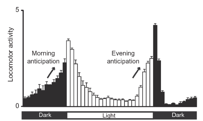
Figure 7.1: Fly activity over the day. Adapted from Nicholas R. J Glossop et al 2011. To meassure fly activity each individual fly is monitored either by counting when they cross a red-light bim (regular activity monitors) of by software tracking (flyboxes).
These changes in behavior are govern by changes in gene expression in particular cell-types in the brain called the pace-makers. If we look at gene expression in these cells over the day we will notice that some genes oscillate. Like Clk and tim, the proteins we analyzed in the previous Lab.
In the circadian field time is reported as “hours after the light is ON”. This is zeitgeber time (ZT) and it is useful to have a unified measurement of time. Most animals in labs are kept in 12 hours of light followed by 12 hours of dark. Therefore, ZT0 is the “sunrise” or lights on and ZT12 is lights off in a light/dark (LD)12:12 cycle time.
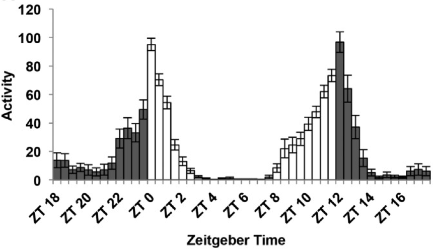
Figure 7.2: Fly activity over the day with ZT scale. Figure adapted from Dubowy et al 2017
As stated before, circadian behaviors is generated by a small subset of neurons.
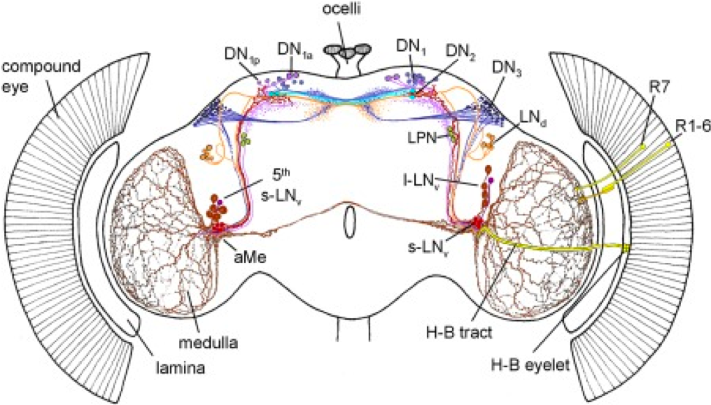
Figure 3.17: Schematic representation of the circadian neural network. Four small ventrolateral neurons (s‐LNvs, red), the 5th s‐LNv (dark violet), four large ventrolateral neurons (l‐LNvs, brown), six dorsolateral neurons (LNds, orange), three lateral posterior neurons (LPN, green), and ca. 60 neurons per hemisphere in three dorsal groups (DN1–3, lilac, cyan, blue, respectively). Adapted from Schubert et al 2018
In the data analyzed in this lab, the authors collected RNA samples over 6 times of the day (ZT3, 7, 11, 15, 19, 23) from 4 cell-types: LNv, LNd, DN1 and Dopaminergic neurons (TH cells). This last group of cells are not part of the circadian core clock but in this study they see oscillating genes!
Packages:
We will use the following packages.
library(ggplot2) #for 2D graph
library(ggrepel) #to get the names in ggplot graph
library(gridExtra) #to arrange the plots
library(factoextra) #extra plots
library(plyr) #table manipulation
library(dplyr)#table manipulation
library(tidyr)#table manipulation
library("RColorBrewer") #extra color palettes
library("pheatmap") #nice heatmaps
library(org.Dm.eg.db) #get annotation
library(MetaCycle) # to identify cycling genes, the successor of JTK according to JTK authors
library(pcaExplorer) #more PCA analysis
7.3 Cycling genes analysis
As stated before, if we want to see cycling we have to look at repetitive patterns in the data cross the day. To determine cycling genes, different approaches can be done. But basically, the idea is to assess for each gene:
1.Identify cycling elements in the data. (ie which genes are changing between the timepoints) 2.If so, in which time point that particular gene has its peak. 3.Which is the amplitude and the period of the cycle: ie. how pronounced is the peak and how often it is cycling.
One popular algorithm used is JTK And its description says: “Its purpose is to identify rhythmic components in large, genome-scale data sets and estimate their period length, phase, and amplitude”
We will use the library: MetaCycle It is the successor of JTK according to JTK authors and it incorporates different approaches:
“Using the same input file, MetaCycle::meta2d implements ARSER (ARS), JTK_CYCLE (JTK) and Lomb-Scargle (LS), from dramatically different disciplines, computer science, statistics and physics, respectively. Three independent algorithms (ARS, JTK and LS) were then selected from best of breed methods (Deckard et al., 2013; Wu et al., 2014). If set analysisStrategy as”auto“(default), it will automatically select proper method from cycMethod for each input dataset”
There is a nice tutorial only from the CRAN repository
And of course you can always use the internal R help ?meta2d
##        Symbol DN1_ZT3_1 DN1_ZT7_1 DN1_ZT11_1 DN1_ZT15_1 DN1_ZT19_1 DN1_ZT23_1
## 1 FBtr0070202         0         0          0          0          0          0
## 2 FBtr0070207         0         0          0          0         14          0
## 3 FBtr0070238         0         0          0          0         21          0
## 4 FBtr0070251         0         0          0          0          0          0
## 5 FBtr0070484         0         0          0          0          0          0
## 6 FBtr0070489         0         0          0          0          0          0
##   DN1_ZT3_2 DN1_ZT7_2 DN1_ZT11_2 DN1_ZT15_2 DN1_ZT19_2 DN1_ZT23_2
## 1         0         0          0          0          0          0
## 2         0         0          0          0         16          7
## 3         0         0          0          0         15          9
## 4         0         0          1          0          2          0
## 5         0         0          0          0          0          1
## 6         0         0          0          0          0          0
This is the raw data, but we should use the normalized one.
##             DN1_ZT3_1 DN1_ZT7_1 DN1_ZT11_1 DN1_ZT15_1 DN1_ZT19_1 DN1_ZT23_1
## FBtr0070202         0         0          0          0   0.000000          0
## FBtr0070207         0         0          0          0   7.039025          0
## FBtr0070238         0         0          0          0  10.558537          0
## FBtr0070251         0         0          0          0   0.000000          0
## FBtr0070484         0         0          0          0   0.000000          0
## FBtr0070489         0         0          0          0   0.000000          0
##             DN1_ZT3_2 DN1_ZT7_2 DN1_ZT11_2 DN1_ZT15_2 DN1_ZT19_2 DN1_ZT23_2
## FBtr0070202         0         0   0.000000          0  0.0000000   0.000000
## FBtr0070207         0         0   0.000000          0  5.6437621  12.719245
## FBtr0070238         0         0   0.000000          0  5.2910269  16.353315
## FBtr0070251         0         0   2.947736          0  0.7054703   0.000000
## FBtr0070484         0         0   0.000000          0  0.0000000   1.817035
## FBtr0070489         0         0   0.000000          0  0.0000000   0.000000
If you read the specifications of meta2d, you need the first column to be the gene name. Lets do it. We can do it wiht base R or with specific packages.
7.3.1 Prepare the tables
We need now to write them in an outside file and run the command. Note that you might be able to use the original data, this is just to keep on learning how to manage the data.
7.3.2 Meta2d
DN1_cyc <- meta2d(infile="cycDN1.csv",filestyle="csv", timepoints=(rep(c(3,7,11,15,19,23),2)),outputFile=FALSE,outRawData=F)## The JTK is in process from 21:14:19 08-30-2020
## Warning: the input 'maxper' is not suitable for JTK, it was reset as 24
## The analysis by JTK is finished at 21:14:45 08-30-2020
## The LS is in process from 21:14:45 08-30-2020
## The analysis by LS is finished at 21:20:08 08-30-2020
## DONE! The analysis about ' cycDN1.csv ' has been finished.
## user.self sys.self elapsed user.child sys.child
## "Time used:" "356.725" "12.003" "370.861" "0" "0"As we can read in the help page ?meta2d the output of this function is:
meta2d will write analysis results in different files under output directory (outdir) if set outputFile = TRUE. Files named with “ARSresult”, “JTKresult” and “LSreult” store analysis results from ARS, JTK and LS respectively. The file named with “meta2d” is the integration file, and it stores integrated values in columns with a common name tag-“meta2d”. The integration file also contains p-value, FDR value, period, phase(adjusted phase if adjustedPhase = “predictedPer”) and amplitude values calculated by each method. If outputFile = FALSE is selected, meta2d will return a list containing the following components:
ARS analysis results from ARS method JTK analysis results from JTK method LS analysis results from LS method meta the integrated analysis results as mentioned above
Let’s explore the results
##         CycID BH.Q ADJ.P PER LAG AMP
## 1 FBtr0070202    1     1   0   0   0
## 2 FBtr0070207    1     1   0   0   0
## 3 FBtr0070238    1     1   0   0   0
## 4 FBtr0070251    1     1   0   0   0
## 5 FBtr0070484    1     1   0   0   0
## 6 FBtr0070489 1 1 0 0 0## CycID PhaseShift PhaseShiftHeight PeakIndex PeakSPD Period p
## 1 FBtr0070202 22.999926 0.000000 NA NA NA 1.0000000
## 2 FBtr0070207 22.999922 6.795629 1 2.5714094 28 0.4706206
## 3 FBtr0070238 22.999926 8.713640 1 2.4520804 28 0.5134413
## 4 FBtr0070251 10.999996 1.473868 48 0.9032149 20 0.9843473
## 5 FBtr0070484 7.721415 0.000000 1 1.2731542 28 0.9277372
## 6 FBtr0070489 22.999926 0.000000 NA NA NA 1.0000000
## N Nindependent Nyquist BH.Q
## 1 12 8 NA 1
## 2 12 8 0.3 1
## 3 12 8 0.3 1
## 4 12 8 0.3 1
## 5 12 8 0.3 1
## 6 12 8 NA 1## CycID JTK_pvalue JTK_BH.Q JTK_period JTK_adjphase JTK_amplitude
## 1 FBtr0070202 1 1 0 NaN 0
## 2 FBtr0070207 1 1 0 NaN 0
## 3 FBtr0070238 1 1 0 NaN 0
## 4 FBtr0070251 1 1 0 NaN 0
## 5 FBtr0070484 1 1 0 NaN 0
## 6 FBtr0070489 1 1 0 NaN 0
## LS_pvalue LS_BH.Q LS_period LS_adjphase LS_amplitude meta2d_pvalue
## 1 1.0000000 1 NA NA 0.000000 1.0000000
## 2 0.4706206 1 28 22.999922 6.795629 0.8253288
## 3 0.5134413 1 28 22.999926 8.713640 0.8557113
## 4 0.9843473 1 20 10.999996 1.473868 0.9998769
## 5 0.9277372 1 28 7.721415 0.000000 0.9973238
## 6 1.0000000 1 NA NA 0.000000 1.0000000
## meta2d_BH.Q meta2d_period meta2d_phase meta2d_Base meta2d_AMP meta2d_rAMP
## 1 1 NA NA 0.0000000 NA NA
## 2 1 28 22.999922 2.4093672 2.81516339 1.16842439
## 3 1 28 22.999926 3.0549360 3.57379221 1.16984191
## 4 1 20 10.999996 0.3720886 0.50175568 0.50175568
## 5 1 28 7.721415 0.1560293 0.07341249 0.07341249
## 6 1 NA NA 0.0000000 NA NAClearly the “meta” is what we want. We can store it in another object to explore it in R or just write a table
DN1_cyc_meta<- as.data.frame(DN1_cyc$meta)

#We will add the gene-names and then export it
DN1_cyc_meta$transcript_name=DN1_cyc_meta$CycID
DN1_cyc_meta=merge(DN1_cyc_meta,annotation_DN1,by="transcript_name")

#the tim, clk and per:
DN1_cyc_meta[which(DN1_cyc_meta$gene_name %in% c("tim","Clk","per")),]
## transcript_name CycID JTK_pvalue JTK_BH.Q JTK_period
## 368 FBtr0070477 FBtr0070477 0.0080482069 0.5867038 24
## 5185 FBtr0076785 FBtr0076785 0.0285920047 0.8536843 20
## 5743 FBtr0077567 FBtr0077567 0.0007025279 0.3232319 20
## 15490 FBtr0100132 FBtr0100132 0.0285920047 0.8536843 20
## 15491 FBtr0100134 FBtr0100134 0.0285920047 0.8536843 20
## 26382 FBtr0332311 FBtr0332311 0.0285920047 0.8536843 24
## 27307 FBtr0333252 FBtr0333252 0.0007025279 0.3232319 20
## 27308 FBtr0333253 FBtr0333253 0.0007025279 0.3232319 20
## 27309 FBtr0333254 FBtr0333254 0.0285920047 0.8536843 24
## 27310 FBtr0333255 FBtr0333255 0.0285920047 0.8536843 24
## 27311 FBtr0333256 FBtr0333256 0.0007025279 0.3232319 20
## 27312 FBtr0333258 FBtr0333258 0.0007025279 0.3232319 20
## 27313 FBtr0333259 FBtr0333259 0.0007025279 0.3232319 20
## JTK_adjphase JTK_amplitude LS_pvalue LS_BH.Q LS_period LS_adjphase
## 368 13 305.3228 0.2045246 1 23.25088 12.95559
## 5185 3 128.3993 0.4297392 1 27.76371 22.99993
## 5743 13 1648.7247 0.0751332 1 23.08772 14.72816
## 15490 3 128.3993 0.4297392 1 27.76371 22.99993
## 15491 3 128.3993 0.4297392 1 27.76371 22.99993
## 26382 13 318.0454 0.3542849 1 23.25088 14.29129
## 27307 13 1648.7247 0.0751332 1 23.08772 14.72816
## 27308 13 1648.7247 0.0751332 1 23.08772 14.72816
## 27309 15 139.8126 0.1773643 1 22.15488 15.32424
## 27310 15 139.8126 0.1773643 1 22.15488 15.32424
## 27311 13 1648.7247 0.0751332 1 23.08772 14.72816
## 27312 13 1648.7247 0.0751332 1 23.08772 14.72816
## 27313 13 1648.7247 0.0751332 1 23.08772 14.72816
## LS_amplitude meta2d_pvalue meta2d_BH.Q meta2d_period meta2d_phase
## 368 724.5210 0.0121962439 1.0000000 23.62544 12.98070
## 5185 488.6181 0.0663405962 1.0000000 23.88186 23.62413
## 5743 4366.7125 0.0005726614 0.4069818 21.54386 13.87341
## 15490 488.6181 0.0663405962 1.0000000 23.88186 23.62413
## 15491 488.6181 0.0663405962 1.0000000 23.88186 23.62413
## 26382 790.6228 0.0566482210 1.0000000 23.62544 13.65932
## 27307 4366.7125 0.0005726614 0.4069818 21.54386 13.87341
## 27308 4366.7125 0.0005726614 0.4069818 21.54386 13.87341
## 27309 320.8403 0.0318683270 1.0000000 23.07744 15.19288
## 27310 320.8403 0.0318683270 1.0000000 23.07744 15.19288
## 27311 4366.7125 0.0005726614 0.4069818 21.54386 13.87341
## 27312 4366.7125 0.0005726614 0.4069818 21.54386 13.87341
## 27313 4366.7125 0.0005726614 0.4069818 21.54386 13.87341
## meta2d_Base meta2d_AMP meta2d_rAMP gene_name
## 368 404.2411 310.1832 0.7673221 per
## 5185 428.9183 455.0223 1.0608602 Clk
## 5743 1976.0053 1791.7205 0.9067387 tim
## 15490 428.9183 455.0223 1.0608602 Clk
## 15491 428.9183 455.0223 1.0608602 Clk
## 26382 420.1319 314.4002 0.7483370 per
## 27307 1976.0053 1791.7205 0.9067387 tim
## 27308 1976.0053 1791.7205 0.9067387 tim
## 27309 150.3703 156.7295 1.0422898 tim
## 27310 150.3703 156.7295 1.0422898 tim
## 27311 1976.0053 1791.7205 0.9067387 tim
## 27312 1976.0053 1791.7205 0.9067387 tim
## 27313 1976.0053 1791.7205 0.9067387 timExport the results in a table
7.3.3 Plot the data.
This it really useful to make plots. We will use the object created before.
genes.cyc = DN1_cyc_meta$gene_name[c(DN1_cyc_meta$JTK_pvalue<0.05 & DN1_cyc_meta$JTK_amplitude>128.3)]#you can put here as many genes as you want, I am seleceting genes with amplitud bigger than clock (Clk)

#I pick the first 8 genes, but you can look at all of them.
ggplot(toplot[toplot$gene_name %in% genes.cyc[1:8] ,],aes(x = as.numeric(ztime),y = value,color=gene_name,shape=rep)) + geom_point() + geom_line() 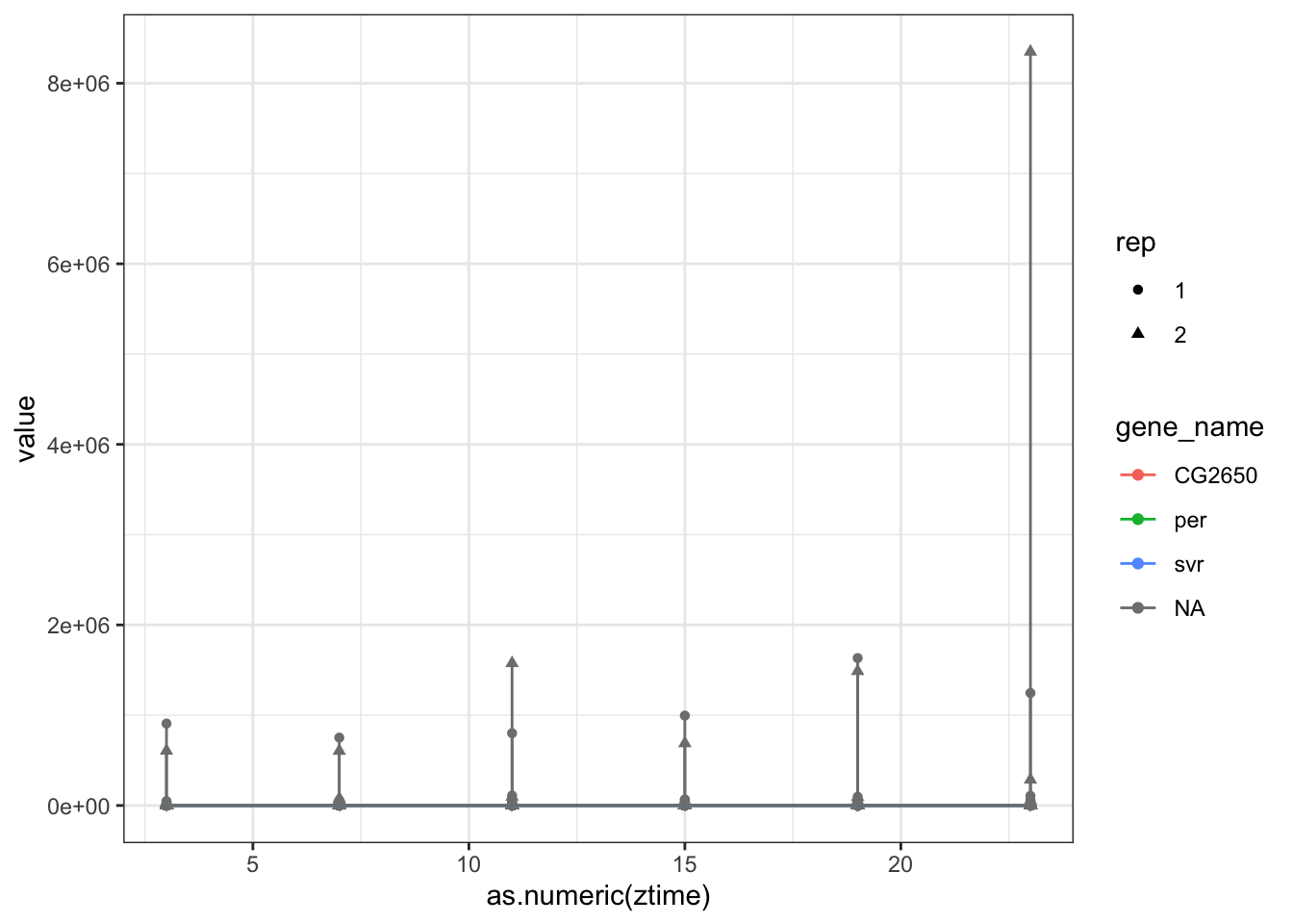
Figure 7.3: Cycling genes.
ggplot(toplot[toplot$gene_name %in% genes.cyc[1:8] ,],aes(x =ztime_2,y = value,color=gene_name,shape=rep)) + geom_point() + geom_line()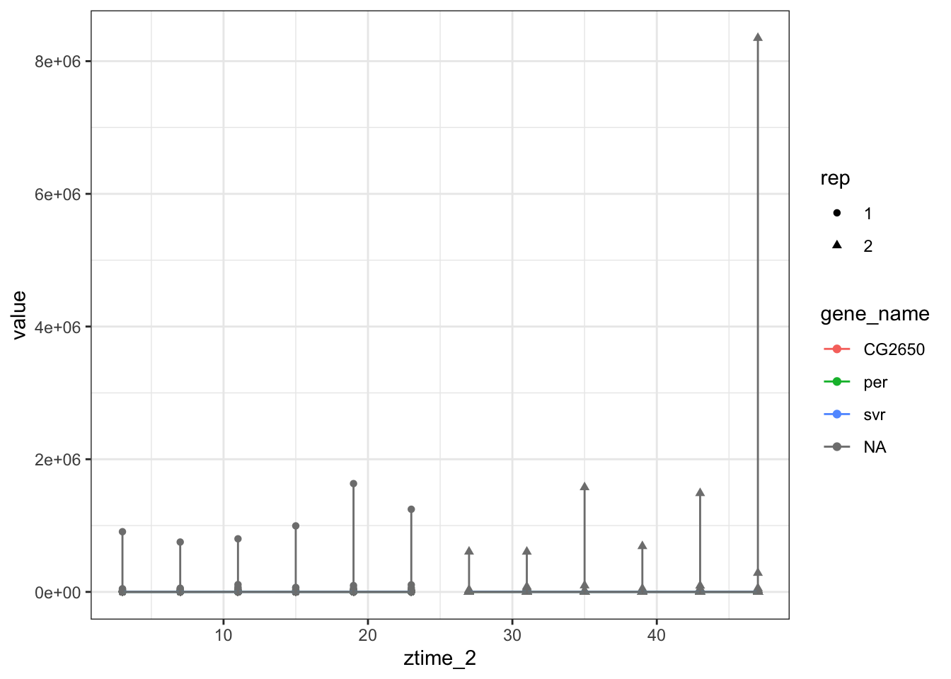
Figure 7.4: Cycling genes.
ggplot(toplot[toplot$gene_name %in% genes.cyc[1:8] ,],aes(x =ztime_2,y = value,color=gene_name,shape=rep)) + geom_point() + geom_line() + facet_wrap(scales = "free",facets = ~gene_name )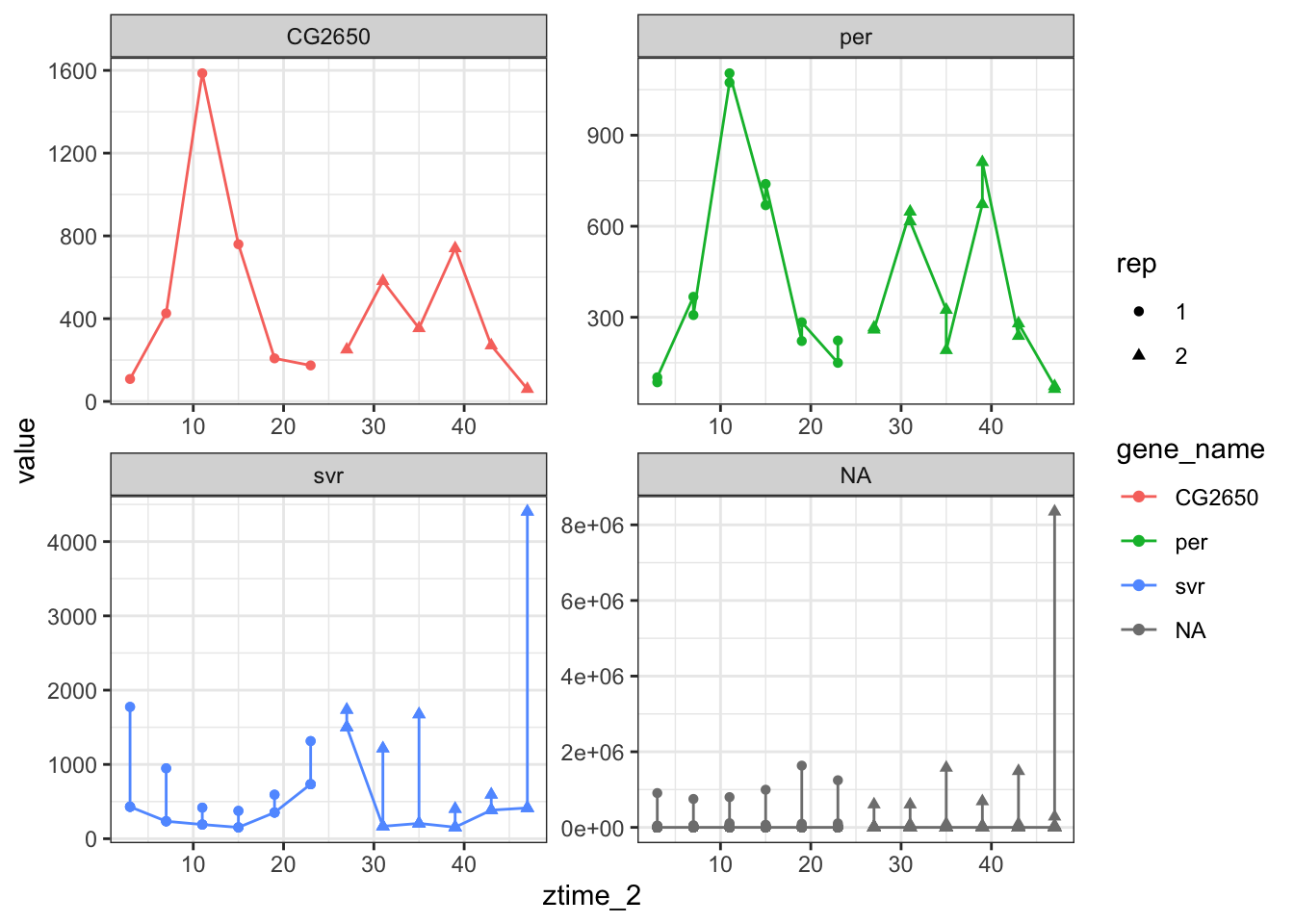
Figure 7.5: Cycling genes.
7.4 Cycling genes analysis normalizing by maximum
This is a more complex set-up I arrived after many trials this is way I found to get more reliable results:
Before doing the analysis, I normalize the expression by the maximum level in each replicate. This mean that for all the replicates the levels will be between 0 and 1. I calculate the amplitude manually: this is just Maximum/Minimum.
I share here some of the code to do it.
- Remove the genes that are all zeros
x<-DN1_gene_expression_norm # copy the DeSeq2 normalized reads

ind=apply(x[-1], 1, function(x)(sum(x)>0)) # remove the genes that are not expressed at all
x=x[ind,]

names(x)
## [1] "Genes" "DN1_ZT3_1" "DN1_ZT7_1" "DN1_ZT11_1" "DN1_ZT15_1"
## [6] "DN1_ZT19_1" "DN1_ZT23_1" "DN1_ZT3_2" "DN1_ZT7_2" "DN1_ZT11_2"
## [11] "DN1_ZT15_2" "DN1_ZT19_2" "DN1_ZT23_2"- Separate by replicate
- Normalization by max
x1<-t(apply((x1[,-1]), 1, function(x)(x/max(x)))) #this is the function that normalize each gene by its maximum
x1<-cbind(as.data.frame(x$Gene),x1)
names(x1)[1]="Gene"
x2<-t(apply((x2[,-1]), 1, function(x)(x/max(x))))- Bind the replicates and run the meta2d
x<-cbind(x1,x2)
x<-x[complete.cases(x),]

write.table(x, file="normtomax.csv", row.names=FALSE,sep = ",")

# Extract the times from the colnames
timepoints=as.numeric(gsub(pattern = "ZT", replacement = "", sapply(strsplit(names(x)[-1],"_"),"[[",2)))

DN1_cyc_norm <-meta2d(infile="normtomax.csv",filestyle="csv", timepoints=timepoints,outputFile=FALSE,outRawData=F)

DN1_cyc_norm_meta2d <- as.data.frame(DN1_cyc_norm$meta)
## The JTK is in process from 21:20:39 08-30-2020
## Warning: the input 'maxper' is not suitable for JTK, it was reset as 24
## The analysis by JTK is finished at 21:21:01 08-30-2020
## The LS is in process from 21:21:01 08-30-2020
## The analysis by LS is finished at 21:25:12 08-30-2020
## DONE! The analysis about ' normtomax.csv ' has been finished.
## user.self sys.self elapsed user.child sys.child
## "Time used:" "279.973" "10.08" "293.003" "0" "0"- Calculate the amplitude manually for each replicate
For this, create a function that merge the results from the cycling analysis and the read counts and calculates the amplitude manually.
mean_nona=function(x){
  mean(x,na.rm =TRUE)
}

merge_counts=function(cyc,cs){

  cs$mean.exp=apply(cs[,-c(1)],1,mean_nona)
  cs=cs[order(cs$Gene),]
  cyc=cyc[order(cyc$CycID),]
  print(unique(cyc$CycID==cs$Gene)) #make sure the we are merging the same genes
  cyc<-cbind(cyc, cs)

  toMatch <- c("_1", "_2")
  cyc$zero=(apply((cyc)[,grep(paste(toMatch,collapse="|"),names(cyc))],1,function(x)(length(which(x %in% 0))>1)))
  cyc=cyc[cyc$zero==F,]

  cyc$AMP_1=(apply((cyc)[,grep("_1",names(cyc))],1,function(x)(1/min(x)))) # amplitude for replicate 1
  cyc$AMP_2=(apply((cyc)[,grep("_2",names(cyc))],1,function(x)(1/min(x)))) # amplitude for replicate 2
  cyc$AMP_min=(apply((cyc)[,grep("^AMP",names(cyc))],1,function(x)(min(x)))) # get the minimum amplitude
  cyc$AMP_min[cyc$AMP_min=="Inf"]=10 # if the minimum is infinite (ie the minimum is cero), I set an arbitrary amplitude

  return(cyc)
}

DN1_cyc_norm_meta2d_mergecounts<-merge_counts(cyc = DN1_cyc_norm_meta2d,cs = x)
## [1] TRUE7.5 Activity
Finish the analysis for the other cell-types. Find a way to compare the results (hint: look at dendrograms) Plot the data for the results of the normalized expression.
7.6 Resources and Bibliography
Dubowy C, Sehgal A. Circadian Rhythms and Sleep in Drosophila melanogaster. Genetics. 2017;205(4):1373-1397. doi:10.1534/genetics.115.185157
MEIRELES-FILHO, Antonio Carlos Alves and KYRIACOU, Charalambos Panayiotis. Circadian rhythms in insect disease vectors. Mem. Inst. Oswaldo Cruz [online]. 2013, vol.108, suppl.1 [cited 2020-07-08], pp.48-58.
Abruzzi KC, Zadina A, Luo W, Wiyanto E, Rahman R, Guo F, et al. (2017) RNA-seq analysis of Drosophila clock and non-clock neurons reveals neuron-specific cycling and novel candidate neuropeptides. PLoS Genet 13(2): e1006613. https://doi.org/10.1371/journal.pgen.1006613
Schubert FK, Hagedorn N, Yoshii T, Helfrich-Förster C, Rieger D. Neuroanatomical details of the lateral neurons of Drosophila melanogaster support their functional role in the circadian system. J Comp Neurol. 2018;526(7):1209-1231. doi:10.1002/cne.24406
DeSeq2 documentations: http://bioconductor.org/packages/release/bioc/vignettes/DESeq2/inst/doc/DESeq2.html
Introduction to implementation steps of MetaCycle Gang Wu, Ron Anafi, Michael Hughes, Karl Kornacker, and John Hogenesch 2015-12-04 https://cran.r-project.org/web/packages/MetaCycle/vignettes/implementation.html
Gene Ontology overview http://geneontology.org/docs/ontology-documentation/